Day 2: Manipulating Data

Last updated on 2026-05-22 | Edit this page

Estimated time: 180 minutes

Overview

Questions

How can I select specific columns or rows from a data frame?
How can I combine multiple data manipulation steps efficiently?
How can I create new columns, summarize data, and reshape data frames?
How do I handle dates in R and export data to a file?

Objectives

Describe the purpose of the dplyr and tidyr packages.
Select certain columns in a data frame with the dplyr function select.
Select certain rows in a data frame according to filtering conditions with the dplyr function filter.
Link the output of one dplyr function to the input of another function with the ‘pipe’ operator |>.
Add new columns to a data frame that are functions of existing columns with mutate.
Use the split-apply-combine concept for data analysis.
Use summarize, group_by, and count to split a data frame into groups of observations, apply summary statistics for each group, and then combine the results.
Describe the concept of a wide and a long table format and for which purpose those formats are useful.
Describe what key-value pairs are.
Format dates.
Reshape a data frame from long to wide format and back with the pivot_wider and pivot_longer commands from the tidyr package.
Export a data frame to a .csv file.

Data Manipulation using `dplyr` and `tidyr`

Packages in R are basically sets of additional functions that let you do more stuff. The functions we’ve been using so far, like str() or data.frame(), come built into R; packages give you access to more of them. Before you use a package for the first time you need to install it on your machine, and then you should import it in every subsequent R session when you need it. You should already have installed the tidyverse package. This is an “umbrella-package” that installs several packages useful for data analysis which work together well such as tidyr, dplyr, ggplot2, tibble, etc.

The tidyverse package tries to address 3 common issues that arise when doing data analysis with some of the functions that come with R:

The results from a base R function sometimes depend on the type of data.
Using R expressions in a non standard way, which can be confusing for new learners.
Hidden arguments, having default operations that new learners are not aware of.

If we haven’t already done so, we can type install.packages("tidyverse") straight into the console. In fact, it’s better to write this in the console than in our script for any package, as there’s no need to re-install packages every time we run the script.

Then, to load the package type:

R

## load the tidyverse packages, incl. dplyr
library(tidyverse)

Getting started with Tidyverse

We’ll read in our data using the read_csv() function, from the tidyverse package readr, instead of read.csv().

R

surveys <- read_csv("data_raw/portal_data_joined.csv")

You will see the message Parsed with column specification, followed by each column name and its data type. When you execute read_csv on a data file, it looks through the first 1000 rows of each column and guesses the data type for each column as it reads it into R. For example, in this dataset, read_csv reads weight as col_double (a numeric data type), and species as col_character. You have the option to specify the data type for a column manually by using the col_types argument in read_csv.

R

## inspect the data
str(surveys)

R

## preview the data
View(surveys)

Notice that the class of the data is now tbl_df

This is referred to as a “tibble”. Tibbles tweak some of the behaviors of the data frame objects we introduced in the previous lesson. The data structure is very similar to a data frame. For our purposes the only difference is that, in addition to displaying the data type of each column under its name, it only prints the first few rows of data and only as many columns as fit on one screen.

What are `dplyr` and `tidyr`?

The package dplyr provides easy tools for the most common data manipulation tasks, built to work directly with data frames.

The package tidyr addresses the common problem of wanting to reshape your data for plotting and use by different R functions. Sometimes we want data sets where we have one row per measurement. Sometimes we want a data frame where each measurement type has its own column, and rows are instead more aggregated groups (e.g., a time period, an experimental unit like a plot or a batch number). Moving back and forth between these formats is non-trivial, and tidyr gives you tools for this and more sophisticated data manipulation.

Callout

Note

An additional feature of dplyr is the ability to work directly with data stored in an external database. The benefits of doing this are that the data can be managed natively in a relational database, queries can be conducted on that database, and only the results of the query are returned. This addresses a common problem with R in that all operations are conducted in-memory and thus the amount of data you can work with is limited by available memory. The database connections essentially remove that limitation in that you can connect to a database of many hundreds of GB, conduct queries on it directly, and pull back into R only what you need for analysis.

To learn more about dplyr and tidyr after the workshop, you may want to check out this handy data transformation with dplyr cheatsheet and this one about tidyr.

Discussion

Stretch Challenge (Difficult - 30 mins)

Install and load dplyr and tidyr within your project environment. This is great for making your code reproducible. You can do this using the package renv.

If you have more packages loaded, filter and select from dplyr can be overwritten by functions of the same name in different packages. Use dplyr::select or prioritize() from the package needs to ensure you’re using the correct version of the function.

Managing Data with dplyr

We’re going to learn some of the most common dplyr functions:

select(): subset columns
filter(): subset rows on conditions
mutate(): create new columns by using information from other columns
group_by() and summarize(): create summary statistics on grouped data
arrange(): sort results
count(): count discrete values

Selecting columns and filtering rows

To select columns of a data frame, use select(). The first argument to this function is the data frame (surveys), and the subsequent arguments are the columns to keep.

R

select(surveys, plot_id, species_id, weight)

To select all columns except certain ones, put a “-” in front of the variable to exclude it.

R

select(surveys, -record_id, -species_id)

This will select all the variables in surveys except record_id and species_id.

To choose rows based on a specific criterion, use filter():

R

filter(surveys, year == 1995)

Pipes

What if you want to select and filter at the same time? There are three ways to do this: use intermediate steps, nested functions, or pipes.

With intermediate steps, you create a temporary data frame and use that as input to the next function, like this:

R

surveys2 <- filter(surveys, weight < 5)
surveys_sml <- select(surveys2, species_id, sex, weight)

This is readable, but can clutter up your workspace with lots of objects that you have to name individually. With multiple steps, that can be hard to keep track of.

You can also nest functions (i.e. one function inside of another), like this:

R

surveys_sml <- select(filter(surveys, weight < 5), species_id, sex, weight)

This is handy, but can be difficult to read if too many functions are nested, as R evaluates the expression from the inside out (in this case, filtering, then selecting).

The last, and best, option is to use pipes. Pipes let you take the output of one function and send it directly to the next, which is useful when you need to do many things to the same dataset. Pipes in R look like |> and are included in base R (a recent addition).

Note: You may also see the older version of the pipe which looks like %>% and is made available via the magrittr package, installed automatically with dplyr. For our purposes, these pipes do the same thing.

R

surveys |>
  filter(weight < 5) |>
  select(species_id, sex, weight)

In the above code, we use the pipe to send the surveys dataset first through filter() to keep rows where weight is less than 5, then through select() to keep only the species_id, sex, and weight columns. Since |> takes the object on its left and passes it as the first argument to the function on its right, we don’t need to explicitly include the data frame as an argument to the filter() and select() functions any more.

Some may find it helpful to read the pipe like the word “then”. For instance, in the above example, we took the data frame surveys, then we filter-ed for rows with weight < 5, then we selected columns species_id, sex, and weight. The dplyr functions by themselves are somewhat simple, but by combining them into linear workflows with the pipe, we can accomplish more complex manipulations of data frames.

If we want to create a new object with this smaller version of the data, we can assign it a new name:

R

surveys_sml <- surveys |>
  filter(weight < 5) |>
  select(species_id, sex, weight)

surveys_sml

Note that the final data frame is the leftmost part of this expression.

Challenge

Using pipes, subset the surveys data to include animals collected before 1995 and retain only the columns year, sex, and weight.

Show me the solution

R

surveys |>
  filter(year < 1995) |>
  select(year, sex, weight)

Challenge

Stretch Challenge (Intermediate - 15 mins)

Create surveys_final using as few lines of code as possible and using pipes to remove the intermediary variables.

R

surveys_2 <- filter(surveys, year > 2000)
surveys_3 <- filter(surveys_2, year != 2001)
surveys_4 <- filter(surveys_3, plot_type == 'Control')
surveys_5 <- select(surveys_4, record_id, month, day, year, sex, weight)
surveys_final <- select(surveys_5, -day)

Show me the solution

R

surveys_final <- surveys |>
  filter(year > 2000, year != 2001, plot_type == 'Control') |>
  select(record_id, month, year, sex, weight)

Mutate

Frequently you’ll want to create new columns based on the values in existing columns, for example to do unit conversions, or to find the ratio of values in two columns. For this we’ll use mutate().

To create a new column of weight in kg:

R

surveys |>
  mutate(weight_kg = weight / 1000)

You can also create a second new column based on the first new column within the same call of mutate():

R

surveys |>
  mutate(weight_kg = weight / 1000,
         weight_lb = weight_kg * 2.2)

If this runs off your screen and you just want to see the first few rows, you can use a pipe to view the head() of the data. (Pipes work with non-dplyr functions, too, as long as the dplyr or magrittr package is loaded).

R

surveys |>
  mutate(weight_kg = weight / 1000) |>
  head()

The first few rows of the output are full of NAs, so if we wanted to remove those we could insert a filter() in the chain:

R

surveys |>
  filter(!is.na(weight)) |>
  mutate(weight_kg = weight / 1000) |>
  head()

is.na() is a function that determines whether something is an NA. The ! symbol negates the result, so we’re asking for every row where weight is not an NA.

Challenge

Create a new data frame from the surveys data that meets the following criteria: contains only the species_id column and a new column called hindfoot_cm containing the hindfoot_length values converted to centimeters. In this hindfoot_cm column, there are no NAs and all values are less than 3. Assume hindfoot_length is currently in mm.

Hint: think about how the commands should be ordered to produce this data frame!

Show me the solution

R

surveys_hindfoot_cm <- surveys |>
  filter(!is.na(hindfoot_length)) |>
  mutate(hindfoot_cm = hindfoot_length / 10) |>
  filter(hindfoot_cm < 3) |>
  select(species_id, hindfoot_cm)

Challenge

Stretch Challenge (Difficult - 20 mins)

Create a new dataframe fom the surveys data with a new column called weight_simplified which has the value 1 if weight is less than or equal to the mean weight and 2 if the weight is more than the mean weight.
What’s the name of the function in dplyr which both selects and mutates? Have a look at the documentation for dplyr

Show me the solution

R

surveys_simplified <- surveys |>
  mutate(weight_simplified =
    ifelse(weight <= mean(weight, na.rm = TRUE), 1, 2))

transmute

Split-Apply-Combine Data Analysis

Many data analysis tasks can be approached using the split-apply-combine paradigm: split the data into groups, apply some analysis to each group, and then combine the results. dplyr makes this very easy through the use of the group_by() function.

The `group_by` and`summarize()` Functions

group_by() is often used together with summarize(), which collapses each group into a single-row summary of that group. group_by() takes as arguments the column names that contain the categorical variables for which you want to calculate the summary statistics. So to compute the mean weight by sex:

R

surveys |>
  group_by(sex) |>
  summarize(mean_weight = mean(weight, na.rm = TRUE))

You may also have noticed that the output from these calls doesn’t run off the screen anymore. It’s one of the advantages of tbl_df over data frame.

You can also group by multiple columns:

R

surveys |>
  group_by(sex, species_id) |>
  summarize(mean_weight = mean(weight, na.rm = TRUE)) |>
  tail()

Here, we used tail() to look at the last six rows of our summary. Before, we had used head() to look at the first six rows. We can see that the sex column contains NA values because some animals had escaped before their sex and body weights could be determined. The resulting mean_weight column does not contain NA but NaN (which refers to “Not a Number”) because mean() was called on a vector of NA values while at the same time setting na.rm = TRUE. To avoid this, we can remove the missing values for weight before we attempt to calculate the summary statistics on weight. Because the missing values are removed first, we can omit na.rm = TRUE when computing the mean:

R

surveys |>
  filter(!is.na(weight)) |>
  group_by(sex, species_id) |>
  summarize(mean_weight = mean(weight))

Here, again, the output from these calls doesn’t run off the screen anymore. If you want to display more data, you can use the print() function at the end of your chain with the argument n specifying the number of rows to display:

R

surveys |>
  filter(!is.na(weight)) |>
  group_by(sex, species_id) |>
  summarize(mean_weight = mean(weight)) |>
  print(n = 15)

Once the data are grouped, you can also summarize multiple variables at the same time (and not necessarily on the same variable). For instance, we could add a column indicating the minimum weight for each species for each sex:

R

surveys |>
  filter(!is.na(weight)) |>
  group_by(sex, species_id) |>
  summarize(mean_weight = mean(weight),
            min_weight = min(weight))

It is sometimes useful to rearrange the result of a query to inspect the values. For instance, we can sort on min_weight to put the lighter species first:

R

surveys |>
  filter(!is.na(weight)) |>
  group_by(sex, species_id) |>
  summarize(mean_weight = mean(weight),
            min_weight = min(weight)) |>
  arrange(min_weight)

To sort in descending order, we need to add the desc() function. If we want to sort the results by decreasing order of mean weight:

R

surveys |>
  filter(!is.na(weight)) |>
  group_by(sex, species_id) |>
  summarize(mean_weight = mean(weight),
            min_weight = min(weight)) |>
  arrange(desc(mean_weight))

Counting

When working with data, we often want to know the number of observations found for each factor or combination of factors. For this task, dplyr provides count(). For example, if we wanted to count the number of rows of data for each sex, we would do:

R

surveys |>
    count(sex)

The count() function is shorthand for something we’ve already seen: grouping by a variable, and summarizing it by counting the number of observations in that group. In other words, surveys |> count() is equivalent to:

R

surveys |>
    group_by(sex) |>
    summarize(count = n())

For convenience, count() provides the sort argument:

R

surveys |>
    count(sex, sort = TRUE)

Previous example shows the use of count() to count the number of rows/observations for one factor (i.e., sex). If we wanted to count combination of factors, such as sex and species, we would specify the first and the second factor as the arguments of count():

R

surveys |>
  count(sex, species)

With the above code, we can proceed with arrange() to sort the table according to a number of criteria so that we have a better comparison. For instance, we might want to arrange the table above in (i) an alphabetical order of the levels of the species and (ii) in descending order of the count:

R

surveys |>
  count(sex, species) |>
  arrange(species, desc(n))

From the table above, we may learn that, for instance, there are 75 observations of the albigula species that are not specified for its sex (i.e. NA).

Challenge

Counting, Grouping and Summarising

How many animals were caught in each plot_type surveyed?
Use group_by() and summarize() to find the mean, min, and max hindfoot length for each species (using species_id). Also add the number of observations (hint: see ?n).
What was the heaviest animal measured in each year? Return the columns year, genus, species_id, and weight.

Show me the solution

R

surveys |>
  count(plot_type)

R

surveys |>
  filter(!is.na(hindfoot_length)) |>
  group_by(species_id) |>
  summarize(
    mean_hindfoot_length = mean(hindfoot_length),
    min_hindfoot_length = min(hindfoot_length),
    max_hindfoot_length = max(hindfoot_length),
    n = n() )

R

surveys |>
  filter(!is.na(weight)) |>
  group_by(year) |>
  filter(weight == max(weight)) |>
  select(year, genus, species, weight) |>
  arrange(year)

Formatting Dates

One of the most common issues that new (and experienced!) R users have is converting date and time information into a variable that is appropriate and usable during analyses. As a reminder from earlier in this lesson, the best practice for dealing with date data is to ensure that each component of your date is stored as a separate variable. Using str(), We can confirm that our data frame has a separate column for day, month, and year, and that each contains integer values.

R

str(surveys)

We are going to use the ymd() function from the package lubridate (which belongs to the tidyverse; learn more here). When you load the tidyverse (library("tidyverse")), the core packages get loaded. lubridate however does not belong to the core tidyverse, so you have to load it explicitly with library(lubridate)

Start by loading the required package:

R

library("lubridate")

ymd() takes a vector representing year, month, and day, and converts it to a Date vector. Date is a class of data recognized by R as being a date and can be manipulated as such. The argument that the function requires is a character vector formatted as “YYYY-MM-DD”.

Let’s create a date object and inspect the structure:

R

my_date <- ymd("2015-01-01")
str(my_date)

Now let’s paste the year, month, and day separately - we get the same result:

R

# sep indicates the character to use to separate each component
my_date <- ymd(paste("2015", "1", "1", sep = "-"))
str(my_date)

We can apply this operation to each row of the surveys dataset. We extract the vectors surveys$year, surveys$month, and surveys$day. Using paste() we can combine these vectors into a new vector for character dates.

R

dates_char_vec <- paste(surveys$year, surveys$month, surveys$day, sep = "-")

This character vector can be used as the argument for ymd():

R

date_vec <- ymd(dates_char_vec)

Something went wrong lets use summary to inspect date_vec:

R

summary(date_vec)

OUTPUT

     Min.      1st Qu.       Median         Mean      3rd Qu.         Max.
"1977-07-16" "1984-03-12" "1990-07-22" "1990-12-15" "1997-07-29" "2002-12-31"
         NA's
        "129"

Some dates have missing values. Let’s investigate where they are coming from.

R

missing_dates_vec <- dates_char_vec[is.na(date_vec)]
head(missing_dates_vec)

OUTPUT

[1] "2000-9-31" "2000-4-31" "2000-4-31" "2000-4-31" "2000-4-31" "2000-9-31"

R

missing_dates_tab <- surveys[is.na(date_vec), c("year", "month", "day")]
head(missing_dates_tab)

OUTPUT

      year month day
 3144 2000     9  31
 3817 2000     4  31
 3818 2000     4  31
 3819 2000     4  31
 3820 2000     4  31
 3856 2000     9  31

Why did these dates fail to parse? If you had to use these data for your analyses, how would you deal with this situation?

Callout

Note

If the data is to be discarded we can use the not logical operator ! to make a filter for the bad dates.

R

date_vec_cleaned <- date_vec[!is.na(date_vec)]

However for now we will include the bad dates and can us this simple filter later if needed.

The resulting Date vector date_vec can be added to surveys as a new column called date:

R

surveys$date <- date_vec
str(surveys) # notice the new column, with 'date' as the class

OUTPUT

 'data.frame': 34786 obs. of  14 variables:
  $ record_id      : int  1 72 224 266 349 363 435 506 588 661 ...
  $ month          : int  7 8 9 10 11 11 12 1 2 3 ...
  $ day            : int  16 19 13 16 12 12 10 8 18 11 ...
  $ year           : int  1977 1977 1977 1977 1977 1977 1977 1978 1978 1978 ...
  $ plot_id        : int  2 2 2 2 2 2 2 2 2 2 ...
  $ species_id     : chr  "NL" "NL" "NL" "NL" ...
  $ sex            : chr  "M" "M" "" "" ...
  $ hindfoot_length: int  32 31 NA NA NA NA NA NA NA NA ...
  $ weight         : int  NA NA NA NA NA NA NA NA 218 NA ...
  $ genus          : chr  "Neotoma" "Neotoma" "Neotoma" "Neotoma" ...
  $ species        : chr  "albigula" "albigula" "albigula" "albigula" ...
  $ taxa           : chr  "Rodent" "Rodent" "Rodent" "Rodent" ...
  $ plot_type      : chr  "Control" "Control" "Control" "Control" ...
  $ date           : Date, format: "1977-07-16" "1977-08-19" ...

Callout

Note

For completeness sake it is worth noting that the above could be achieved in one line. surveys$date <- ymd(paste(surveys$year, surveys$month, surveys$day, sep = "-")) However, we would again see the warning and could inspect it like so: summary(surveys$date) head(surveys[is.na(surveys$date), , c("year", "month", "day")]) This way the r environment is kept cleaner however it is more difficult to unpick where errors have occured.

Reshaping with pivot_wider and pivot_longer

In surveys, the rows of surveys contain the values of variables associated with each record (the unit), values such as the weight or sex of each animal associated with each record. What if instead of comparing records, we wanted to compare the different mean weight of each genus between plots? (Ignoring plot_type for simplicity).

We’d need to create a new table where each row (the unit) is comprised of values of variables associated with each plot. In practical terms this means the values in genus would become the names of column variables and the cells would contain the values of the mean weight observed on each plot.

Having created a new table, it is therefore straightforward to explore the relationship between the weight of different genera within, and between, the plots. The key point here is that we are still following a tidy data structure, but we have reshaped the data according to the observations of interest: average genus weight per plot instead of recordings per date.

The opposite transformation would be to transform column names into values of a variable.

We can do both these of transformations with two tidyr functions, pivot_longer() and pivot_wider().

Pivot_wider

pivot_wider() takes three principal arguments:

the data
names_from indicates which column (or columns) to get the name of the output column from
values_from indicates which column (or columns) to get the cell values from

Further arguments include values_fill which, if set, fills in missing values with the value provided.

Let’s use pivot_wider() to transform surveys to find the mean weight of each genus in each plot over the entire survey period. We use filter(), group_by() and summarize() to filter our observations and variables of interest, and create a new variable for the mean_weight.

R

surveys_gw <- surveys |>
  filter(!is.na(weight)) |>
  group_by(plot_id, genus) |>
  summarize(mean_weight = mean(weight))

str(surveys_gw)

This yields surveys_gw where the observations for each plot are spread across multiple rows, 196 observations of 3 variables. Using pivot_wider() with names_from genus and values_from mean_weight this becomes 24 observations of 11 variables, one row for each plot.

R

surveys_wide<- surveys_gw |>
  pivot_wider(names_from = genus, values_from = mean_weight)

str(surveys_wide)

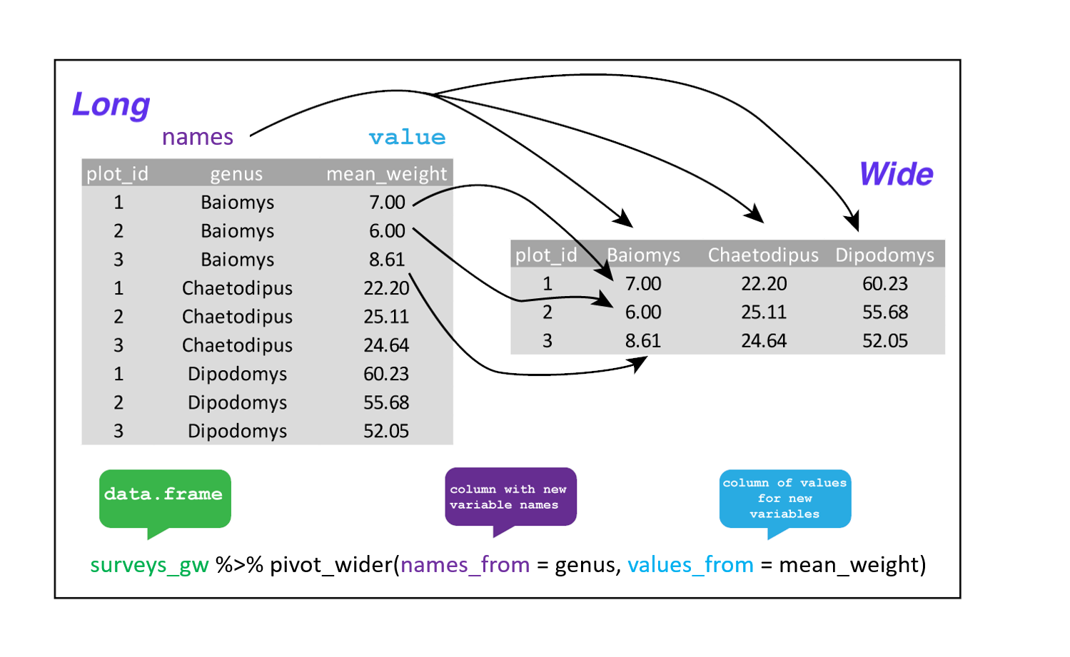
Diagram illustrating the pivot_wider transformation.

We could now plot comparisons between the weight of genera in different plots, although we may wish to fill in the missing values first.

R

surveys_gw |>
  pivot_wider(names_from = genus, values_from = mean_weight, values_fill = 0) |>
  head()

Pivot_longer

The opposing situation could occur if we had been provided with data in the form of surveys_wide, where the genus names are column names, but we wish to treat them as values of a genus variable instead.

In this situation we are gathering the column names and turning them into a pair of new variables. One variable represents the column names as values, and the other variable contains the values previously associated with the column names.

pivot_longer() takes four principal arguments:

the data
cols indicates the columns to pivot into longer format (or those not to pivot)
names_to indicates the name of the column to create from the data stored in the column names of data.
values_to indicates the name of the column to create from the data stored in cell values.

To recreate surveys_gw from surveys_wide we would set names_to genus and values_to mean_weight and use all columns except plot_id for the key variable. Here we exclude plot_id from being pivoted.

R

surveys_long <- surveys_wide |>
  pivot_longer(cols = -plot_id, names_to = "genus", values_to = "mean_weight")

str(surveys_long)

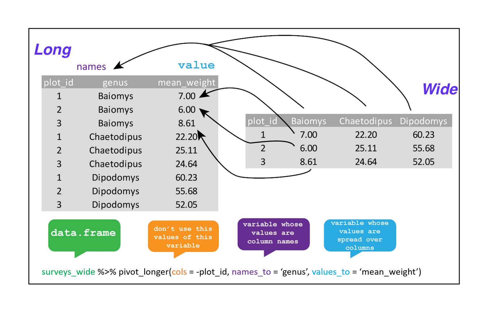
Diagram illustrating the pivot_longer transformation.

Note that now the NA genera are included in the new pivot_longer format. Using pivot_wider and then pivot_longer can be a useful way to balance out a dataset so every replicate has the same composition.

We could also have used a specification for what columns to include. This can be useful if you have a large number of identifying columns, and it’s easier to specify what to pivot than what to leave alone. And if the columns are directly adjacent, we don’t even need to list them all out - just use the : operator!

R

surveys_wide |>
  pivot_longer(cols = Baiomys:Spermophilus, names_to = "genus", values_to = "mean_weight") |>
  head()

Challenge

The surveys data set has two measurement columns: hindfoot_length and weight. This makes it difficult to do things like look at the relationship between mean values of each measurement per year in different plot types. Let’s walk through a common solution for this type of problem.

Use pivot_longer() to create a dataset where we have a key column called measurement and a value column that takes on the value of either hindfoot_length or weight. Hint: You’ll need to specify which columns are being pivoted.
With this new data set, calculate the average of each measurement in each year for each different plot_type. Then pivot_wider() them into a data set with a column for hindfoot_length and weight. Hint: You only need to specify the name and value columns for pivot_wider().

Show me the solution

R

surveys_long <- surveys |>
  pivot_longer(cols = c(hindfoot_length, weight), names_to ='measurement', values_to = 'value')

R

surveys_long |>
  group_by(year, measurement, plot_type) |>
  summarize(mean_value = mean(value, na.rm=TRUE)) |>
  pivot_wider(names_from = measurement, values_from = mean_value)

Exporting data

Now that you have learned how to use dplyr to extract information from or summarize your raw data, you may want to export these new data sets to share them with your collaborators or for archival.

Similar to the read_csv() function used for reading CSV files into R, there is a write_csv() function that generates CSV files from data frames.

Before using write_csv(), we are going to create a new folder, data, in our working directory that will store this generated dataset. We don’t want to write generated datasets in the same directory as our raw data. It’s good practice to keep them separate. The data_raw folder should only contain the raw, unaltered data, and should be left alone to make sure we don’t delete or modify it. In contrast, our script will generate the contents of the data directory, so even if the files it contains are deleted, we can always re-generate them.

In preparation for our next lesson on plotting, we are going to prepare a cleaned up version of the data set that doesn’t include any missing data.

Let’s start by removing observations of animals for which weight and hindfoot_length are missing, or the sex has not been determined:

R

surveys_complete <- surveys |>
  filter(!is.na(weight),           # remove missing weight
         !is.na(hindfoot_length),  # remove missing hindfoot_length
         !is.na(sex))                # remove missing sex

Because we are interested in plotting how species abundances have changed through time, we are also going to remove observations for rare species (i.e., that have been observed less than 50 times). We will do this in two steps: first we are going to create a data set that counts how often each species has been observed, and filter out the rare species; then, we will extract only the observations for these more common species:

R

## Extract the most common species_id
species_counts <- surveys_complete |>
    count(species_id) |>
    filter(n >= 50)

## Only keep the most common species
surveys_complete <- surveys_complete |>
  filter(species_id %in% species_counts$species_id)

To make sure that everyone has the same data set, check that surveys_complete has 30463 rows and 13 columns by typing dim(surveys_complete).

Now that our data set is ready, we can save it as a CSV file in our data folder.

R

write_csv(surveys_complete, file = "data/surveys_complete.csv")

Discussion

Stretch Challenge (Fiendish - 45 mins)

Data can also be imported and exported in the form of binary files. Have a look at documentation for the readBin() and writeBin() functions, as well as this helpful guide to binary files in r. Then try to export the surveys data as a binary file before importing the binary file back into r.

Key Points

dplyr is a package for making tabular data manipulation easier and tidyr reshapes data so that it is in a convenient format for plotting or analysis. They are both part of the tidyverse package.
A subset of columns from a dataframe can be selected using select().
To choose rows based on a specific criterion, use filter().
Pipes let you take the output of one function and send it directly to the next, which is useful when you need to do many things to the same dataset.
To create new columns based on the values in existing columns, use mutate().
Many data analysis tasks can be approached using the split-apply-combine paradigm: split the data into groups, apply some analysis to each group, and then combine the results. This can be achieved using the group_by() and summarize() functions.
Dates can be formatted using the package ‘lubridate’.
To reshape data between wide and long formats, use pivot_wider() and pivot_longer() from the tidyr package.
Export data from a dataframe to a csv file using write_csv().

Day 2: Manipulating Data

Overview

Questions

Objectives

Data Manipulation using dplyr and tidyr

R

Getting started with Tidyverse

R

R

R

What are dplyr and tidyr?

Note

Stretch Challenge (Difficult - 30 mins)

Managing Data with dplyr

Selecting columns and filtering rows

R

R

R

Pipes

R

R

R

R

Challenge

Show me the solution

R

Stretch Challenge (Intermediate - 15 mins)

R

Show me the solution

R

Mutate

R

R

R

R

Challenge

Show me the solution

R

Stretch Challenge (Difficult - 20 mins)

Show me the solution

R

Split-Apply-Combine Data Analysis

The group_by andsummarize() Functions

R

R

R

R

R

R

R

Counting

R

R

R

R

R

Counting, Grouping and Summarising

Show me the solution

R

R

R

Formatting Dates

R

R

R

R

R

R

R

OUTPUT

R

OUTPUT

R

OUTPUT

Note

R

R

OUTPUT

Note

Reshaping with pivot_wider and pivot_longer

Data Manipulation using `dplyr` and `tidyr`

What are `dplyr` and `tidyr`?

The `group_by` and`summarize()` Functions