
Random Forests
Last updated on 2026-06-23 | Edit this page
Overview
Questions
- What are random forests?
- How do random forests improve decision tree models?
Objectives
- Introduce random forests.
- Use random forests for classification and regression models.
- Evaluate the quality of a random forest model.
We saw in the previous episode that decision tree models can be sensitive to small changes in the training data. Random Forests mitigate this issue by forming an ensemble (i.e., set) of decision trees, and using them all together to make a prediction.
Wine Dataset
For this episode, we will use a data set described in the article
Modeling wine preferences by data mining from physicochemical
properties, in Decision Support Systems, 47(4):547-553, by P.
Cortez, A. Cerdeira, F. Almeida, T. Matos and J. Reis. (Instructions for
downloading this data set are in the setup
page.) The data set contains quality ratings and measurements from
6497 samples of wine; rows 1:1599 are red wine samples, and
rows 1600:6497 are white wine.
R
library(tidyverse)
library(here)
wine <- read_csv(here("data", "wine.csv"))
R
glimpse(wine)
ggplot(wine, aes(x = quality)) +
  geom_histogram(binwidth = 1)
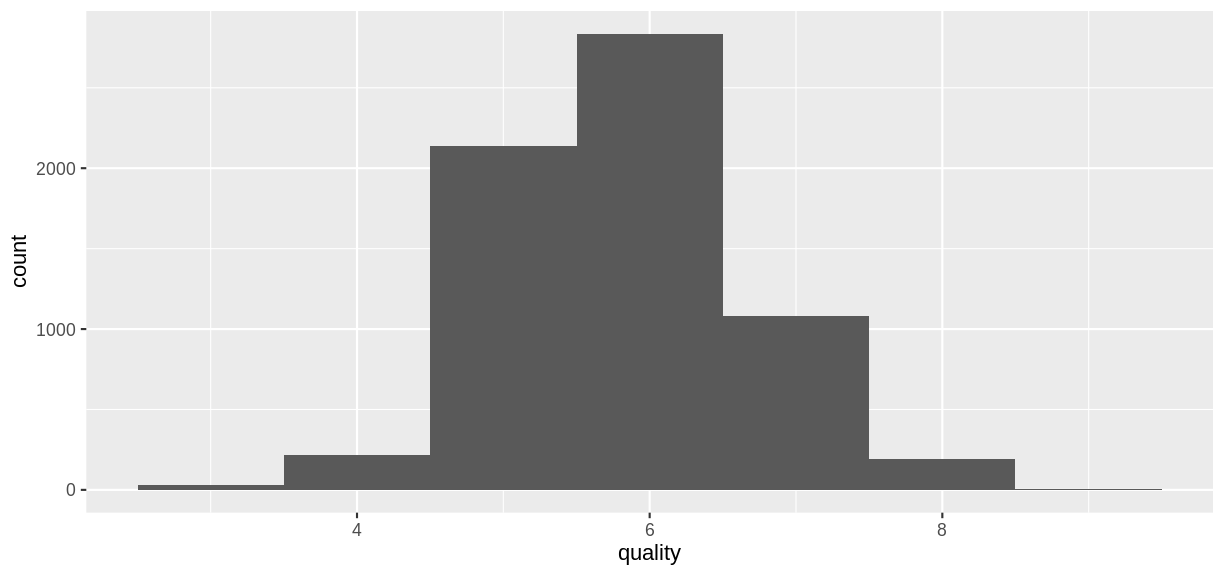
The goal of the models that follow will be to predict the
quality rating of a wine sample from its chemical
properties.
Red Wine Classification Model
To illustrate classification models with this data set, let’s create
a categorical variable grade that will serve as a response
variable.
R
redwineClass <- wine |>
  slice(1:1599) |>  # just the red wine samples
  mutate(grade = as_factor(if_else(quality < 5.5, "bad", "good"))) |>
  select(-quality) # get rid of the quality variable
summary(redwineClass$grade)
OUTPUT
 bad good
 744  855
Create Training and Test Sets
Create training and test sets using an 80/20 split.
R
trainSize <- round(0.80 * nrow(redwineClass))
set.seed(1234)
trainIndex <- sample(nrow(redwineClass), trainSize)
trainDF <- redwineClass |>
  slice(trainIndex)
testDF <- redwineClass |>
  slice(-trainIndex)
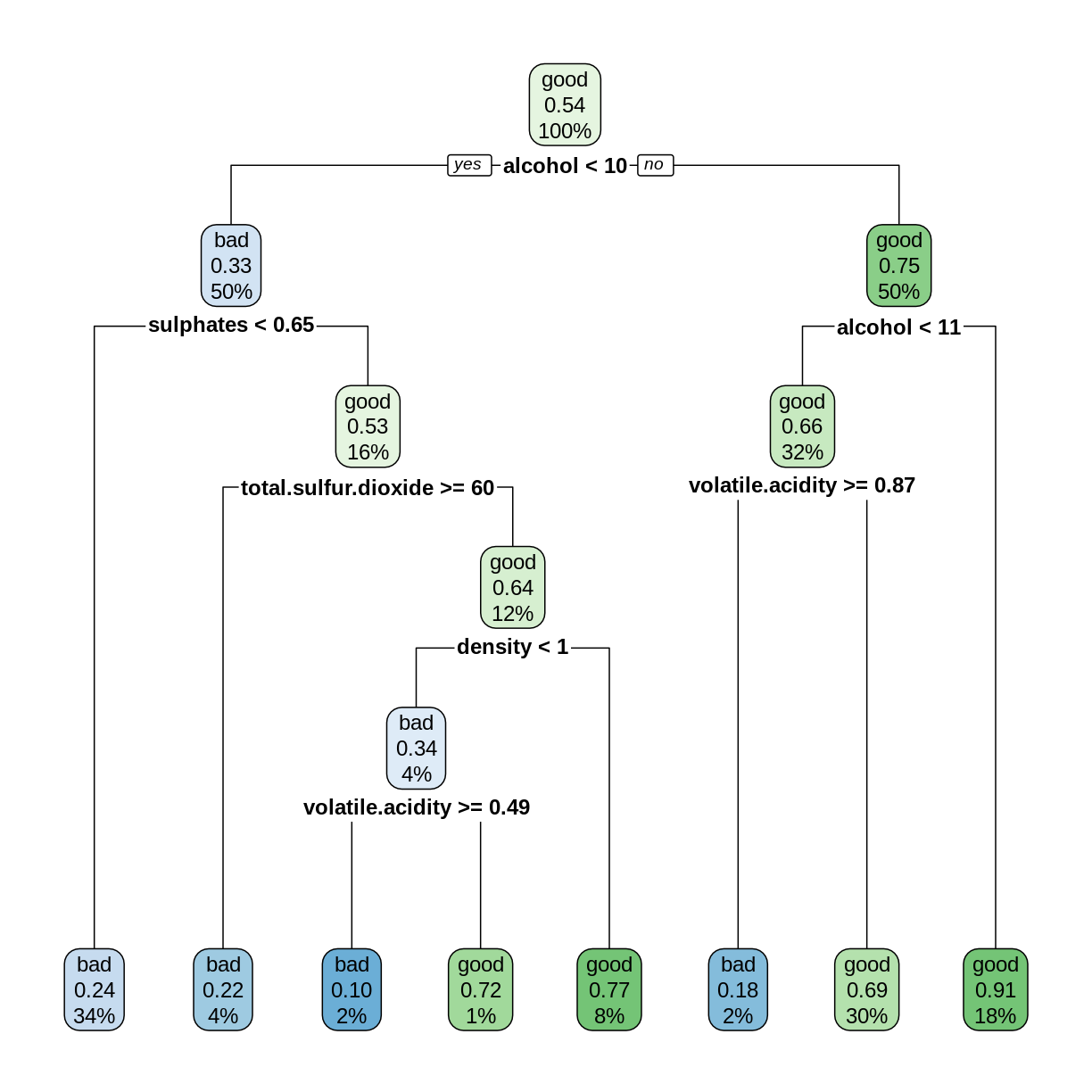
Challenge: Create a decision tree model
Use the rpart function to create a decision tree model
for predicting the grade variable from the remaining
columns in the redwineClass data frame. Use the training
and testing sets defined above. Compute the testing set accuracy.
R
library(rpart)
library(rpart.plot)
rwTree <- rpart(grade ~ ., data = trainDF)
rpart.plot(rwTree)
R
predMatrix <- predict(rwTree, testDF)
predDF <- testDF |>
  bind_cols(predMatrix)
predictedGrade <- ifelse(predDF$bad > 0.5, "bad", "good")
accuracy <- sum(testDF$grade == predictedGrade)/nrow(testDF)
OUTPUT
[1] 0.696875The decision tree model can correctly predict the grade about 70% of the time.
Random Forest Classification Model
A random forest model combines several decision tree models as follows.
- Several different decision trees are built, each from a random bootstrap sample of the same size as the original data. This process is also known as bagging (bootstrap aggregation).
- For each tree model, a randomly-chosen subset of variables is chosen to determine each split.
- Each decision tree model makes a prediction, and the category with the most “votes” is selected as the prediction of the random forest.
More details can be found in Breiman’s 2002 paper, pages 8-9.
The randomForest package is an R implementation of
Breiman and Cutler’s original Fortran code. The syntax for building a
model is similar to lm, glm, and
rpart. Because of the randomness used in the algorithm, it
is good practice to set the random seed so that the results will be
reproducible.
R
library(randomForest)
set.seed(4567)
redwineForest <- randomForest(grade ~ ., data = trainDF)
The predict function works on random forests. Observe
that it returns a vector of levels of the grade
variable.
R
rwpred2 <- predict(redwineForest, testDF)
head(rwpred2)
OUTPUT
  1   2   3   4   5   6
bad bad bad bad bad bad
Levels: bad goodChallenge: Accuracy of the Random Forest Model
Compute the testing set accuracy of the random forest model above. Compare this accuracy with the decision tree model in the previous challenge.
R
sum(testDF$grade == rwpred2)/nrow(testDF)
OUTPUT
[1] 0.821875The random forest model can correctly predict the grade about 82% of the time, which is an improvement of about 12 percentage points over the decision tree model.
Out-of-bag Error
Since each tree in the random forest is built on a bootstrap sample
of the rows in the training set, some rows will be left out of each
sample. Each tree can then make a prediction on each row that was
excluded, i.e., “out of the bag” (OOB). Each row will be excluded by
several trees, which form a subforest that produces an aggregate
prediction for each row. The out-of-bag estimate of the error
rate is the error rate of these predictions. The OOB error rate gives a
convenient estimate of the error rate of the model (error = 1 -
accuracy). The print function reports the OOB error.
R
print(redwineForest)
OUTPUT
Call:
 randomForest(formula = grade ~ ., data = trainDF)
               Type of random forest: classification
                     Number of trees: 500
No. of variables tried at each split: 3

        OOB estimate of  error rate: 19.16%
Confusion matrix:
     bad good class.error
bad  470  119   0.2020374
good 126  564   0.1826087
The confusion matrix gives further details on how the OOB error was calculated: Out of 470+119 bad wines, 119 were classified as good, and out of 126+564 good wines, 126 were classified as bad. Check that (119+126)/(470+119+126+564) = 0.1916.
Train on the whole data set
Given that OOB error gives us a good way to estimate model accuracy, we can train random forest models on the entire data set, without using a train/test split (Breiman, 2001, p. 8).
R
set.seed(4567)
rwforFull <- randomForest(grade ~ ., data = redwineClass)
print(rwforFull)
OUTPUT
Call:
 randomForest(formula = grade ~ ., data = redwineClass)
               Type of random forest: classification
                     Number of trees: 500
No. of variables tried at each split: 3

        OOB estimate of  error rate: 16.82%
Confusion matrix:
     bad good class.error
bad  615  129   0.1733871
good 140  715   0.1637427
Caveat: If you plan to “tune” your model by adjusting the
optional parameters in randomForest, it is still good
practice to set aside a testing set for assessing model accuracy after
the model has been tuned using only the training data. A train/test
split is also helpful if you want to compare random forest models with
other types of models.
Variable Importance
The out-of-bag errors can also be used to assess the importance of
each explanatory variable in contributing to the accuracy of the model.
If we set importance = TRUE in a call to
randomForest, the function will keep track of how much the
OOB accuracy decreases when each variable is randomly permuted.
Scrambling a variable in this way effectively removes its predictive
power from the model, so we would expect the most important variables to
have the greatest decreases in accuracy.
R
set.seed(2345)
rwforFull <- randomForest(grade ~ ., data = redwineClass, importance = TRUE)
importance(rwforFull, type = 1)
OUTPUT
                     MeanDecreaseAccuracy
fixed.acidity                    33.60865
volatile.acidity                 50.37700
citric.acid                      30.12944
residual.sugar                   31.40780
chlorides                        34.39463
free.sulfur.dioxide              32.60753
total.sulfur.dioxide             50.95265
density                          42.35901
pH                               36.46366
sulphates                        58.41187
alcohol 75.06260Challenge: Most and Least Important
Based on the Mean Decrease in Accuracy, Which two variables are the most important, and which two are the least important? Are these results consistent with the decision tree model you constructed in the first challence of this episode?
For convenience, let’s sort the rows of the importance matrix.
R
importance(rwforFull, type = 1) |>
  as_tibble(rownames = "Variable") |>
  arrange(desc(MeanDecreaseAccuracy))
OUTPUT
# A tibble: 11 × 2
   Variable             MeanDecreaseAccuracy
   <chr>                               <dbl>
 1 alcohol                              75.1
 2 sulphates                            58.4
 3 total.sulfur.dioxide                 51.0
 4 volatile.acidity                     50.4
 5 density                              42.4
 6 pH                                   36.5
 7 chlorides                            34.4
 8 fixed.acidity                        33.6
 9 free.sulfur.dioxide                  32.6
10 residual.sugar                       31.4
11 citric.acid                          30.1
The top two variables are alcohol and
sulphates, which both occur near the root of the decision
tree. The least important variables are residual.sugar and
citric.acid, which do not occur in the decision tree. So it
seems consistent that the important variables play important roles in
the decision tree, while the unimportant variables do not.
Red Wine Regression Model
So far, we have applied decision trees and random forests to classification problems, where the dependent variable is categorical. These techniques also apply to regression problems, where we are predicting a quantitative variable.
Recall that in the original wine data set, there is a
variable called quality that assigns each sample a
numerical quality score. For the examples that follow, we will treat
quality as a quantitative variable. As before, we select
the rows that contain observations of red wines, and we form training
and testing sets.
R
redwine <- wine |> slice(1:1599)
trainSize <- round(0.80 * nrow(redwine))
set.seed(1234)
trainIndex <- sample(nrow(redwine), trainSize)
trainDF <- redwine |>
  slice(trainIndex)
testDF <- redwine |>
  slice(-trainIndex)
Fit a Decision Tree
When the dependent variable is quantitative, we use the
method = "anova" option in rpart to construct
a decision tree. In this situation, the predicted value corresponding to
each node is the mean value of the observations assigned to the node,
and the algorithm searches for a split that minimizes the sum of the
squared errors of these predictions.
R
rwtree <- rpart(quality ~ ., data = trainDF, method = "anova")
rpart.plot(rwtree)
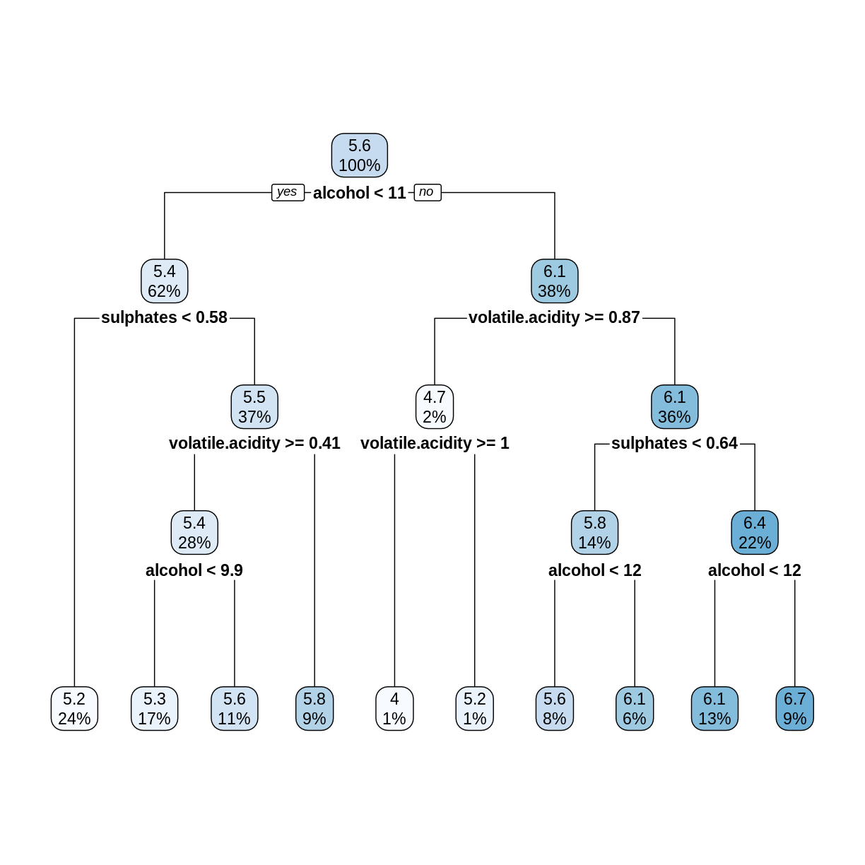
The rpart.plot command rounds off numerical values to
save space. To see more digits of accuracy, print the tree in text
format.
R
rwtree
OUTPUT
n= 1279

node), split, n, deviance, yval
      * denotes terminal node

 1) root 1279 827.94210 5.636435
   2) alcohol< 10.525 787 332.33800 5.364676
     4) sulphates< 0.575 310 100.56770 5.154839 *
     5) sulphates>=0.575 477 209.24950 5.501048
      10) volatile.acidity>=0.405 364 149.63460 5.403846
        20) alcohol< 9.85 223  66.76233 5.278027 *
        21) alcohol>=9.85 141  73.75887 5.602837 *
      11) volatile.acidity< 0.405 113  45.09735 5.814159 *
   3) alcohol>=10.525 492 344.51020 6.071138
     6) volatile.acidity>=0.8725 26  23.11538 4.730769
      12) volatile.acidity>=1.015 10   6.00000 4.000000 *
      13) volatile.acidity< 1.015 16   8.43750 5.187500 *
     7) volatile.acidity< 0.8725 466 272.07730 6.145923
      14) sulphates< 0.635 184  95.77717 5.831522
        28) alcohol< 11.65 102  53.84314 5.627451 *
        29) alcohol>=11.65 82  32.40244 6.085366 *
      15) sulphates>=0.635 282 146.24470 6.351064
        30) alcohol< 11.55 166  79.81325 6.138554 *
        31) alcohol>=11.55 116  48.20690 6.655172 *
For example, the first split tests whether
alcohol < 10.525, not 11 as shown in the plot of the
tree.
Challenge: Check the Splits
In the above decision tree, consider the root (5.6), its left child
(5.4), and the leftmost leaf (5.2). Check that these numbers are in fact
the average quality values (rounded to one decimal place)
of the observations in trainDF that are assigned to each
node.
The root node contains all the observations, so compute its mean
quality value.
R
mean(trainDF$quality)
OUTPUT
[1] 5.636435The left child of the root contains observations where
alcohol is less than 10.525.
R
trainDF |>
  filter(alcohol < 10.525) |>
  summarize(nodeValue = mean(quality))
OUTPUT
# A tibble: 1 × 1
  nodeValue
      <dbl>
1      5.36
The leftmost leaf contains observations where alcohol is
less than 10.525 and sulphates is less than 0.575.
R
trainDF |>
  filter(alcohol < 10.525, sulphates < 0.575) |>
  summarize(nodeValue = mean(quality))
OUTPUT
# A tibble: 1 × 1
  nodeValue
      <dbl>
1      5.15
Decision Tree RMSE
For regression trees, each leaf is assigned a predicted value, and
the predict function selects the appropriate
leaf/prediction based on the values of the explanatory variables.
R
predictedQuality <- predict(rwtree, testDF)
head(predictedQuality)
OUTPUT
       1        2        3        4        5        6
5.154839 5.278027 5.278027 5.154839 5.154839 5.602837
Since this is a regression model, we assess its performance using the root mean squared error (RMSE).
R
errors <- predictedQuality - testDF$quality
decTreeRMSE <- sqrt(mean(errors^2))
decTreeRMSE
OUTPUT
[1] 0.6862169Random Forest Regression Model
Constructing a random forest regression model uses
randomForest with the same syntax as we used for
classification models. The only difference is that the response variable
quality in our formula is a quantitative variable. The
predicted values given by predict are the average
predictions of all the trees in the forest.
R
set.seed(4567)
rwfor <- randomForest(quality ~ ., data = trainDF)
predQualRF <- predict(rwfor, testDF)
rfErrors <- predQualRF - testDF$quality
rfRMSE <- sqrt(mean(rfErrors^2))
rfRMSE
OUTPUT
[1] 0.5913485The random forest RMSE is better (smaller) than the decision tree RMSE.
R
print(rwfor)
OUTPUT
Call:
 randomForest(formula = quality ~ ., data = trainDF)
               Type of random forest: regression
                     Number of trees: 500
No. of variables tried at each split: 3

          Mean of squared residuals: 0.3269279
                    % Var explained: 49.5
The Mean of squared residuals is the MSE of the
out-of-bag errors. The % Var explained term is a “pseudo
R-squared”, computed as 1 - MSE/Var(y). The OOB MSE should be close to
the MSE on the testing set. So again, you don’t always need a train/test
split when working with random forests.
We conclude this episode with a series of challenges.
Challenge: Variable Importance
As with classification models, setting importance = TRUE
in a call to randomForest will use the OOB errors to
measure variable importance. In the regression case, the decrease in
performance when a variable is permuted is measured by the percentage
increase in MSE (%IncMSE). The larger the
%IncMSE, the more important the variable.
Compute the %IncMSE variable importance for the red wine
regression model, and sort the variables by their importance. Re-train
the model on the entire redwine data set instead of on the
testing set. Are the most important variables the same as in the
classification model?
The syntax is almost identical to the classification case. Since the
identifier %IncMSE contains special characters, it must be
enclosed in backticks.
R
set.seed(2345)
rwFull <- randomForest(quality ~ ., data = redwine, importance = TRUE)
importance(rwFull, type = 1) |>
  as_tibble(rownames = "Variable") |>
  arrange(desc(`%IncMSE`))
OUTPUT
# A tibble: 11 × 2
   Variable             `%IncMSE`
   <chr>                    <dbl>
 1 alcohol                   59.2
 2 sulphates                 55.6
 3 volatile.acidity          39.7
 4 total.sulfur.dioxide      38.3
 5 density                   34.5
 6 chlorides                 32.7
 7 free.sulfur.dioxide       30.0
 8 citric.acid               28.9
 9 fixed.acidity             28.4
10 pH                        25.1
11 residual.sugar            24.2
The top five most important variables are the same as in the
classification model, but their order is slightly different. The
variable pH seems to be relatively more important in the
classification model.
Challenge: Linear Regression Model
In Episode 2, we used the lm function to fit a linear
model to the training set, and then we computed the RMSE on the testing
set. Repeat this process for the redwine data set. How does
the linear regression RMSE compare to the random forest RMSE? Compare
the summary of your linear model with the variable
importance rankings from the previous challenge.
R
redwine.lm <- lm(quality ~ ., data = trainDF)
lmRMSE <- sqrt(mean((predict(redwine.lm, testDF) - testDF$quality)^2))
lmRMSE
OUTPUT
[1] 0.6880957The random forest RMSE is less than the linear model RMSE.
R
summary(redwine.lm)
OUTPUT
Call:
lm(formula = quality ~ ., data = trainDF)

Residuals:
     Min       1Q   Median       3Q      Max
-2.68737 -0.36035 -0.03507  0.43456  1.95898

Coefficients:
                       Estimate Std. Error t value Pr(>|t|)
(Intercept)           9.3242378 23.4596015   0.397   0.6911
fixed.acidity         0.0108114  0.0284758   0.380   0.7043
volatile.acidity     -1.2144573  0.1320387  -9.198  < 2e-16 ***
citric.acid          -0.2957551  0.1608745  -1.838   0.0662 .
residual.sugar        0.0193480  0.0168430   1.149   0.2509
chlorides            -1.8858347  0.4583915  -4.114 4.14e-05 ***
free.sulfur.dioxide   0.0054883  0.0023783   2.308   0.0212 *
total.sulfur.dioxide -0.0034664  0.0007974  -4.347 1.49e-05 ***
density              -5.0636470 23.9244350  -0.212   0.8324
pH                   -0.4331191  0.2065623  -2.097   0.0362 *
sulphates             0.9244109  0.1306583   7.075 2.47e-12 ***
alcohol               0.2886439  0.0293633   9.830  < 2e-16 ***
---
Signif. codes:  0 '***' 0.001 '**' 0.01 '*' 0.05 '.' 0.1 ' ' 1

Residual standard error: 0.6385 on 1267 degrees of freedom
Multiple R-squared:  0.3762,	Adjusted R-squared:  0.3708
F-statistic: 69.46 on 11 and 1267 DF,  p-value: < 2.2e-16
The variables with the smallest p-values (Pr(>|t|))
tend to correspond to the most important variables in the random forest
model.
Challenge: White Wine
Rows 1600-6497 of the wine data frame correspond to
white wine observations. Use these rows to train and test a random
forest model, as we did with the red wine observations. Compute a
testing set RMSE, and assess variable importance. Are the important
variables for predicting white wine quality the same as the important
variables for predicting red wine quality?
R
whitewine <- wine |> slice(1600:6497)
trainSize <- round(0.80 * nrow(whitewine))
set.seed(1234)
trainIndex <- sample(nrow(whitewine), trainSize)
trainDF <- whitewine |> dplyr::slice(trainIndex)
testDF <- whitewine |> dplyr::slice(-trainIndex)
wwfor <- randomForest(quality ~ ., data = trainDF)
predQualww <- predict(wwfor, testDF)
errors <- predQualww - testDF$quality
wwRMSE <- sqrt(mean(errors^2))
The RMSE on the white wine testing set is about 0.63.
R
set.seed(4567)
wwforFull <- randomForest(quality ~ ., data = whitewine, importance = TRUE)
importance(wwforFull, type = 1) |>
  as_tibble(rownames = "Variable") |>
  arrange(desc(`%IncMSE`))
Relative to red wine, free.sulfur.dioxide is much more
important for predicting white wine quality, and sulphates
is less important.
- Random forests can make predictions of a categorical or quantitative variable.
- Random forests, with their default settings, work reasonably well.