
Gradient Boosted Trees
Last updated on 2026-06-23 | Edit this page
Estimated time: 70 minutes
Overview
Questions
- What is gradient boosting?
- How can we train an XGBoost model?
- What is the learning rate?
Objectives
- Introduce XGBoost models.
- Train regression models using XGBoost
- Explore the effect of learning rate on the training process.
Gradient Boosted Trees
A random forest is called an ensemble method, because it combines the results of a set of trees to form a single prediction. Gradient boosted trees are also ensemble methods, but instead of forming a forest of trees from different random samples, they grow successive trees that systematically reduce the error of the model at each iteration.
We will be using the R package xgboost, which gives a
fast, scalable implementation of a gradient boosting framework. For more
information on how xgboost works, see the XGBoost
Presentation vignette and the Introduction
to Boosted Trees tutorial in the XGBoost documentation. In this
episode we will use XGBoost to create a regression model, but this
framework can also be used for classification problems.
Reload the Red Wine Data
R
library(tidyverse)
library(here)
R
library(xgboost)
Notice that both xgboost and dplyr have a
function called slice. In the following code block, we
specify that we want to use the dplyr version.
R
wine <- read_csv(here("data", "wine.csv"))
redwine <- wine |> dplyr::slice(1:1599)
trainSize <- round(0.80 * nrow(redwine))
set.seed(1234)
trainIndex <- sample(nrow(redwine), trainSize)
trainDF <- redwine |> dplyr::slice(trainIndex)
testDF <- redwine |> dplyr::slice(-trainIndex)
The xgboost package defines a data structure called
xgb.DMatrix that optimizes storage and retrieval. To use
the advanced features of xgboost, it is necessary to
convert our training and test sets to the xgb.DMatrix
class.
R
dtrain <- xgb.DMatrix(data = as.matrix(select(trainDF, -quality)), label = trainDF$quality)
dtest <- xgb.DMatrix(data = as.matrix(select(testDF, -quality)), label = testDF$quality)
Training an XGBoost Model
Since we specified a label in our dtrain
and dtest matrices, there is no need to specify a formula
when training a model using xgb.train. The label that we
specified (quality rating) will be the response variable, and the
columns of the data that we specified will be the
explanatory variables. One option that we must specify is
nrounds, which restricts the number of boosting iterations
the algorithm will make.
R
redwineXGB <- xgb.train(data = dtrain, nrounds = 10)
Let’s calculate the RMSE on our testing set. The predict
function for XGBoost models expects a matrix, so we pass it the
xgb.DMatrix that we created from our testing set.
R
pQuality <- predict(redwineXGB, dtest)
errors <- pQuality - testDF$quality
sqrt(mean(errors^2)) #RMSE
OUTPUT
[1] 0.6561705More Details on the Training Process
The xgb.train command will automatically calculate the
RMSE on our testing set after each iteration if we set the testing set
in the evals.
R
redwineXGB <- xgb.train(data = dtrain, evals = list(test = dtest), nrounds = 10)
OUTPUT
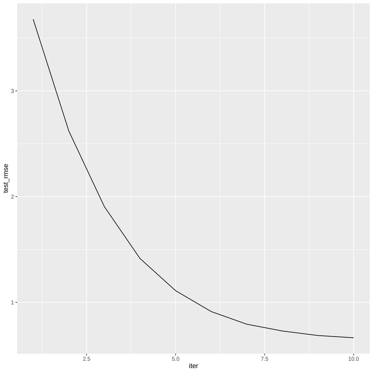
[1]	test-rmse:0.739547
[2]	test-rmse:0.697529
[3]	test-rmse:0.677260
[4]	test-rmse:0.666461
[5]	test-rmse:0.663789
[6]	test-rmse:0.661025
[7]	test-rmse:0.656802
[8]	test-rmse:0.657357
[9]	test-rmse:0.656321
[10]	test-rmse:0.656171
The training history is saved as a data frame in the attribute
evaluation_log, so we can plot how the RMSE changes during
the training process.
R
attr(redwineXGB, "evaluation_log") |>
  ggplot(aes(x = iter, y = test_rmse)) +
  geom_line()
Challenge: How many boosting iterations?
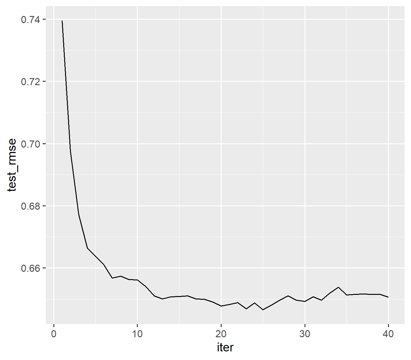
Experiment with different values of nrounds in the above
call to xgb.train. Does the accuracy of the model improve
with more iterations? Is there a point after which the model ceases to
improve?
The accuracy of the model doesn’t appear to improve after iteration 25.
R
redwineXGB <- xgb.train(data = dtrain,
                        evals = list(test = dtest),
                        nrounds = 40)
OUTPUT
[1]	test-rmse:0.739547
[2]	test-rmse:0.697529
[3]	test-rmse:0.677260
[4]	test-rmse:0.666461
[5]	test-rmse:0.663789
[6]	test-rmse:0.661025
[7]	test-rmse:0.656802
[8]	test-rmse:0.657357
[9]	test-rmse:0.656321
[10]	test-rmse:0.656171
[11]	test-rmse:0.654021
[12]	test-rmse:0.651006
[13]	test-rmse:0.650065
[14]	test-rmse:0.650734
[15]	test-rmse:0.650865
[16]	test-rmse:0.651042
[17]	test-rmse:0.650033
[18]	test-rmse:0.649995
[19]	test-rmse:0.649126
[20]	test-rmse:0.647756
[21]	test-rmse:0.648309
[22]	test-rmse:0.648837
[23]	test-rmse:0.646943
[24]	test-rmse:0.648741
[25]	test-rmse:0.646583
[26]	test-rmse:0.648100
[27]	test-rmse:0.649653
[28]	test-rmse:0.651069
[29]	test-rmse:0.649710
[30]	test-rmse:0.649308
[31]	test-rmse:0.650731
[32]	test-rmse:0.649718
[33]	test-rmse:0.651962
[34]	test-rmse:0.653782
[35]	test-rmse:0.651400
[36]	test-rmse:0.651547
[37]	test-rmse:0.651667
[38]	test-rmse:0.651585
[39]	test-rmse:0.651566
[40]	test-rmse:0.650699
R
attr(redwineXGB, "evaluation_log") |>
  ggplot(aes(x = iter, y = test_rmse)) +
  geom_line()
Learning Rate
Machine learning algorithms that reduce a loss function over a sequence of iterations typically have a setting that controls the learning rate. A smaller learning rate will generally reduce the error by a smaller amount at each iteration, and therefore will require more iterations to arrive at a given level of accuracy. The advantage to a smaller learning rate is that the algorithm is less likely to overshoot the optimum fit; the disadvantage is the algorithm may not reach the optimum fit.
In XGBoost, the setting that controls the learning rate is called
eta, which is one of several hyperparameters that
can be adjusted. Its default value is 0.3, but smaller values will
usually perform better. It must take a value in the range 0 <
eta < 1.
The following code will set eta to its default value. We
include a value for early_stopping_rounds, which will halt
the training after a specified number of iterations pass without
improvement. When using early_stopping_rounds,
nrounds can be set to a very large number. To avoid
printing too many lines of output, we also set a value for
print_every_n.
R
redwineXGB <- xgb.train(data = dtrain,
                        params = list(eta = 0.3),
                        evals = list(test = dtest),
                        nrounds = 1000,
                        early_stopping_rounds = 10,
                        print_every_n = 5)
OUTPUT
Will train until test_rmse hasn't improved in 10 rounds.

[1]	test-rmse:0.739547
[6]	test-rmse:0.661025
[11]	test-rmse:0.654021
[16]	test-rmse:0.651042
[21]	test-rmse:0.648309
[26]	test-rmse:0.648100
[31]	test-rmse:0.650731
Stopping. Best iteration:
[35]	test-rmse:0.651400

[35]	test-rmse:0.651400
The output is misleading here as there was no improvement after 10 rounds at iteration 35 but a lower test rmse was seen at iteration 26. You can check the lowest test_rmse definitively by finding the minimum value in the evaluation log:
R
elog <- attr(redwineXGB, "evaluation_log")

elog[which.min(elog$test_rmse), ]
OUTPUT
    iter test_rmse
   <num>     <num>
1: 25 0.6465827Challenge: Experiment with the learning rate.
Experiment with different values of eta in the above
call to xgb.train. Notice how smaller values of eta require
more iterations. Can you find a value of eta that results
in a lower testing set RMSE than the default?
A learning rate around 0.1 reduces the RMSE somewhat.
R
redwineXGB <- xgb.train(data = dtrain,
                        params = list(eta = 0.1),
                        evals = list(test = dtest),
                        nrounds = 1000,
                        early_stopping_rounds = 10,
                        print_every_n = 15)
OUTPUT
Will train until test_rmse hasn't improved in 10 rounds.

[1]	test-rmse:0.789059
[16]	test-rmse:0.643070
[31]	test-rmse:0.629120
[46]	test-rmse:0.625930
Stopping. Best iteration:
[48]	test-rmse:0.625455

[48]	test-rmse:0.625455
R
elog <- attr(redwineXGB, "evaluation_log")

elog[which.min(elog$test_rmse), ]
OUTPUT
    iter test_rmse
   <num>     <num>
1:    38 0.6253475
Variable Importance
As with random forests, you can view the predictive importance of each explanatory variable.
R
xgb.importance(model = redwineXGB)
OUTPUT
                 Feature       Gain      Cover  Frequency
                  <char>      <num>      <num>      <num>
 1:              alcohol 0.30854145 0.20533266 0.08665431
 2:     volatile.acidity 0.14497002 0.12210243 0.10889713
 3:            sulphates 0.12760406 0.13532236 0.08711770
 4: total.sulfur.dioxide 0.08528885 0.10227935 0.09360519
 5:        fixed.acidity 0.06277324 0.06687905 0.14365153
 6:            chlorides 0.05994638 0.08001722 0.09592215
 7:              density 0.04635801 0.06776201 0.07599629
 8:       residual.sugar 0.04470028 0.06218626 0.09267841
 9:          citric.acid 0.04053801 0.06268225 0.08109361
10:                   pH 0.04017616 0.05639794 0.06672845
11:  free.sulfur.dioxide 0.03910355 0.03903844 0.06765524
The rows are sorted by Gain, which measures the accuracy
improvement contributed by a feature based on all the splits it
determines. Note that the sum of all the gains is 1.
Training Error vs. Testing Error
Like many machine learning algorithms, gradient boosting operates by minimizing the error on the training set. However, we evaluate its performance by computing the error on the testing set. These two errors are usually different, and it is not uncommon to have much lower training RMSE than testing RMSE.
To see both training and testing errors, we can add a
train item to the evals.
R
redwineXGB <- xgb.train(data = dtrain,
                        params = list(eta = 0.1),
                        evals = list(train = dtrain, test = dtest),
                        nrounds = 1000,
                        early_stopping_rounds = 10,
                        print_every_n = 15)
OUTPUT
Multiple eval metrics are present. Will use test_rmse for early stopping.
Will train until test_rmse hasn't improved in 10 rounds.

[1]	train-rmse:0.763413	test-rmse:0.789059
[16]	train-rmse:0.467861	test-rmse:0.643070
[31]	train-rmse:0.366838	test-rmse:0.629120
[46]	train-rmse:0.314553	test-rmse:0.625930
Stopping. Best iteration:
[48]	train-rmse:0.311647	test-rmse:0.625455

[48]	train-rmse:0.311647	test-rmse:0.625455
R
attr(redwineXGB, "evaluation_log") |>
  pivot_longer(cols = c(train_rmse, test_rmse), names_to = "RMSE") |>
  ggplot(aes(x = iter, y = value, color = RMSE)) +
  geom_line()
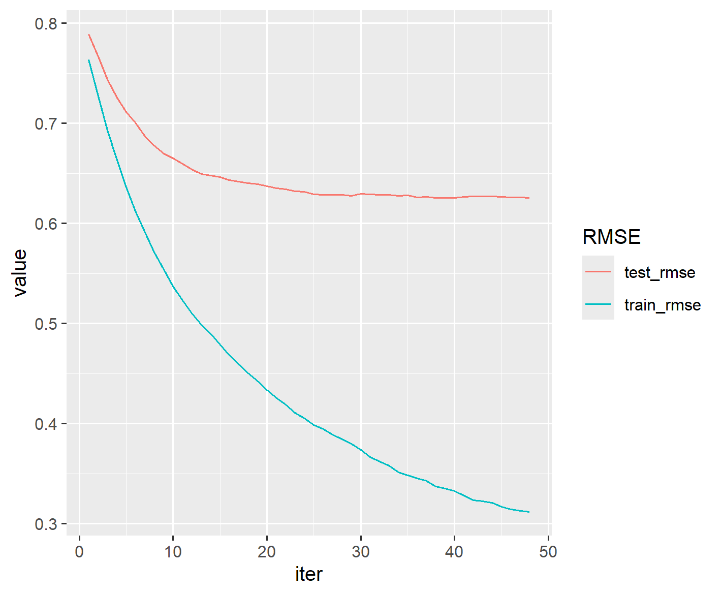
Notice that beyond iteration 20 or so, the training RMSE continues to decrease while the testing RMSE has basically stabilized. This divergence indicates that the later training iterations are improving the model based on the particularities of the training set, but in a way that does not generalize to the testing set.
Saving a trained model
As models become more complicated, the time it takes to train them
becomes nontrivial. For this reason, it can be helpful to save a trained
XGBoost model. We’ll create a directory in our project called
saved_models and save our XGBoost model in a universal
binary format that can be read by any XGBoost interface (e.g., R,
Python, Julia, Scala).
R
dir.create(here("saved_models"))
xgb.save(redwineXGB, here("saved_models", "redwine.model"))
This trained model can be loaded into a future R session with the
xgb.load command.
R
reloaded_model <- xgb.load(here("saved_models", "redwine.model"))
However, while reloaded_model can be used with the
predict function, it is not identical to the
redwineXGB object. For reproducibility, it is important to
save the source code used in the training process.
Challenge: White Wine
Build an XGBoost model for the white wine data (rows 1600-6497) of
the wine data frame. Compare the RMSE and variable
importance with the random forest white wine model from the previous
episode.
R
whitewine <- wine |> dplyr::slice(1600:6497)
trainSize <- round(0.80 * nrow(whitewine))
set.seed(1234)
trainIndex <- sample(nrow(whitewine), trainSize)
trainDF <- whitewine |> dplyr::slice(trainIndex)
testDF <- whitewine |> dplyr::slice(-trainIndex)
dtrain <- xgb.DMatrix(data = as.matrix(select(trainDF, -quality)),
                      label = trainDF$quality)
dtest <- xgb.DMatrix(data = as.matrix(select(testDF, -quality)),
                     label = testDF$quality)
whitewineXGB <- xgb.train(data = dtrain,
                          params = list(eta = 0.1),
                          evals = list(train = dtrain, test = dtest),
                          nrounds = 1000,
                          early_stopping_rounds = 10,
                          print_every_n = 20)
elog <- attr(whitewineXGB, "evaluation_log")
elog[which.min(elog$test_rmse), ]
xgb.importance(model = whitewineXGB)
attr(whitewineXGB, "evaluation_log") |>
  pivot_longer(cols = c(train_rmse, test_rmse), names_to = "RMSE") |>
  ggplot(aes(x = iter, y = value, color = RMSE)) +
  geom_line()
The testing set RMSE (0.66) is worse than what we obtained in the random forest model (0.63). The important explanatory variables are similar.
So far, our XGBoost models have performed slightly worse than the equivalent random forest models. In the next episode we will explore ways to improve these results.
- Gradient boosted trees can be used for the same types of problems that random forests can solve.
- The learning rate can affect the performance of a machine learning algorithm.