Introduction to Job Scheduling
Overview
Teaching: 45 min
Exercises: 30 minQuestions
What is a scheduler and why does a cluster need one?
How do I launch a program to run on a compute node in the cluster?
How do I capture the output of a program that is run on a node in the cluster?
Objectives
Submit a simple script to the cluster using Slurm.
Monitor the execution of jobs using command line tools.
Describe the basic states through which a submitted job progresses to completion or failure.
Inspect the output and error files of your jobs.
Cancel a running job.
Job Scheduler
An HPC system might have thousands of nodes and thousands of users. How do we decide who gets what and when? How do we ensure that a task is run with the resources it needs? This job is handled by a special piece of software called the scheduler. On an HPC system, the scheduler manages which jobs run where and when.
The following illustration compares these tasks of a job scheduler to a waiter in a restaurant. If you can relate to an instance where you had to wait for a while in a queue to get in to a popular restaurant, then you may now understand why sometimes your job does not start instantly as on your laptop.

The scheduler used here is Slurm. Although Slurm is not used everywhere, running jobs is quite similar regardless of what software is being used. The exact syntax might change, but the concepts remain the same.
Running a Batch Job
A Basic Script
The most basic use of the scheduler is to run a command non-interactively. Any command (or series of commands) that you want to run on the cluster is called a job, and the process of using a scheduler to run the job is called batch job submission.
In this case, the job we want to run is a shell script – essentially a text file containing a list of UNIX commands to be executed in a sequential manner. Our shell script will have three parts:
- On the very first line, we’ll add
#!/usr/bin/env bash. The#!(pronounced “hash-bang” or “shebang”) tells the computer what program is meant to process the contents of this file. In this case, we are telling it that the commands that follow are written for the command-line shell (what we’ve been doing everything in so far). - Anywhere below the first line, we’ll add an
echocommand with a friendly greeting. When run, the shell script will print whatever comes afterechoin the terminal.echo -nwill print everything that follows, without ending the line by printing the new-line character.
- On the last line, we’ll invoke the
hostnamecommand, which will print the name of the machine the script is run on.
Let’s use nano to write this script.
[yourUsername@login7a [cosma7] ~]$ nano example-job.sh
#!/usr/bin/env bash

echo -n "This script is running on "
hostname
You can then use Ctrl-O followed by Enter to save the file, and Ctrl-X to exit the editor.
Creating Our Test Job
Run the script. Does it execute on the cluster or just our login node?
Solution
[yourUsername@login7a [cosma7] ~]$ bash example-job.shThis script is running on login7a
Submitting the Job
This script ran on the login node, but we want to take advantage of
the compute nodes: we need the scheduler to queue up example-job.sh
to run on a compute node.
To submit this task to the scheduler, we use the
sbatch command.
This creates a job which will run the script when dispatched to
a compute node which the queuing system has identified as being
available to perform the work.
[yourUsername@login7a [cosma7] ~]$ sbatch example-job.sh
However, running the script in its current form may yield an error like the following:
sbatch: error: A valid account is required (use -A and a DiRAC project or Unix group)
sbatch: error: Batch job submission failed: Unspecified error
In this case, it’s telling us that we need to specify more details for submitting it. As it turns out, as a minimum for COSMA we need to specify the following:
- Our account: this is the systems budgetary account to which we individually are assigned. You can find out the accounts you have access to by using the
sacctmgr list user yourUsernamecommand. - Partition: HPC system resources are typically split by type (such as cpu, gpu, large memory, etc.), or some other classification, into partitions. The configuration of these varies from system to system, but essentially are different queues to which you may submit your job. You may only be authorised to use specific partitions/queues.
- Walltime: the maximum amount of real-world time your job will take to run, specified as
days-hours:minutes:seconds(thedayscan be omitted).
Note that depending on the system, other minimal parameters may also be necessary such as specifying a desired quality of service, or the minimum number of required nodes. But we’ll leave these for now.
We can specify them on the command line when submitting our job, like the following. Our job is very short running, so let’s just give it a maximum wall time of 1 minute:
$ sbatch --account=yourAccount --partition=cosma7 --time=00:01:00 example-job.sh
Submitted batch job 5791510
And that’s what we need to do to submit a job. Our work is done – now the scheduler takes over and tries to run the job for us.
Monitoring our job
While the job is waiting to run, it goes into a list of jobs called the queue.
To check on our job’s status, we check the queue using the command squeue:
[yourUsername@login7a [cosma7] ~]$ squeue -u yourUsername
You may find it looks like this:
  JOBID PARTITION     NAME     USER ST       TIME  NODES NODELIST(REASON)
5791510 cosma7-pa example- yourUser PD       0:00      1 (Priority)
We can see all the details of our job, including the partition, user, and also the state of the job (in the ST column). In this case, we can see it is in the PD or PENDING state. Typically, jobs go through the following states:
PD- pending: sometimes our jobs might need to wait in a queue first before they can be allocated to a node to runR- running: job has an allocation and is currently runningCG- completing: job is in the process of completingCD- completed: the job is completed
You can get a full list of job status codes via the SLURM documentation.
Where’s the Output?
On the login node, this script printed output to the terminal – but now, when
squeueshows the job has finished, nothing was printed to the terminal.Cluster job output is typically redirected to a file in the directory you launched it from. on DiRAC, for example, the output file looks like
slurm-<job_number>.out, with<job_number>representing the unique identifier for the job. Uselsto find andcatto read the file.
Customising a Job
In the job we just ran we didn’t specify any detailed requirements for what our job will need. In a real-world scenario, that’s probably not what we want. Chances are, we will need more cores, more memory, more time, among other special considerations.
So far, we’ve specified job requirements directly on the command line which is quick and convenient, but somewhat limited and less clear when specifying many more parameters. Plus, we may forget which parameters we used in previous runs, which may be critical to reproducing a previous result. The good news is that we can amend our submission script directly to include these parameters instead.
Comments in UNIX shell scripts (denoted by #) are typically ignored, but
there are exceptions. For instance the special #! comment at the beginning of
scripts specifies what program should be used to run it (you’ll typically see
#!/usr/bin/env bash). Schedulers like Slurm also
have a special comment used to denote special scheduler-specific options.
Though these comments differ from scheduler to scheduler,
Slurm’s special comment is #SBATCH. Anything
following the #SBATCH comment is interpreted as an
instruction to the scheduler.
Let’s illustrate this by example. First, we’ll add the account, partition, and time
parameters to the script directly, then give the job itself a different name. By default,
a job’s name is the name of the script, but the --job-name (or -J for short) option
can be used to change the name of a job. Amend the example-job.sh script to look like
the following (amending yourAccount accordingly):
#!/usr/bin/env bash
#SBATCH --account=yourAccount
#SBATCH --partition=cosma7
#SBATCH --time=00:01:00
#SBATCH --job-name=hello-world

echo -n "This script is running on "
hostname
Submit the job and monitor its status:
[yourUsername@login7a [cosma7] ~]$ sbatch example-job.sh
[yourUsername@login7a [cosma7] ~]$ squeue -u yourUsername
  JOBID PARTITION     NAME     USER ST       TIME  NODES NODELIST(REASON)
5791531 cosma7-pa hello-wo yourUser PD       0:00      1 (Priority)
Fantastic, we’ve successfully changed the name of our job!
Resource Requests
What about more important changes, such as the number of cores and memory for our jobs? One thing that is absolutely critical when working on an HPC system is specifying the resources required to run a job, which allows the scheduler to find the right time and place to schedule our job. If you do not specify requirements (such as the amount of time you need), you will likely be stuck with your site’s default resources, which is probably not what you want.
The following are several key resource requests:
-
--ntasks=<ntasks>or-n <ntasks>: How many CPU cores does your job need, in total? -
--mem=<megabytes>: How much memory on a node does your job need in megabytes? You can also specify gigabytes using by adding a little “g” afterwards (example:--mem=5g) -
--nodes=<nnodes>or-N <nnodes>: How many separate machines does your job need to run on? Note that if you setntasksto a number greater than what one machine can offer, Slurm will set this value automatically.
Note that just requesting these resources does not make your job run faster, nor does it necessarily mean that you will consume all of these resources. It only means that these are made available to you. Your job may end up using less memory, or less time, or fewer nodes than you have requested, and it will still run.
It’s best if your requests accurately reflect your job’s requirements. We’ll talk more about how to make sure that you’re using resources effectively in a later episode of this lesson.
Job environment variables
When Slurm runs a job, it sets a number of environment variables for the job. One of these will let us check what directory our job script was submitted from. The
SLURM_SUBMIT_DIRvariable is set to the directory from which our job was submitted. Using theSLURM_SUBMIT_DIRvariable, modify your job so that it prints out the location from which the job was submitted.Solution
[yourUsername@login7a [cosma7] ~]$ nano example-job.sh
[yourUsername@login7a [cosma7] ~]$ cat example-job.sh
#!/usr/bin/env bash #SBATCH --account=yourAccount #SBATCH --partition=cosma7 #SBATCH --time=00:00:30 #SBATCH --job-name=hello-world echo "This job was launched in the following directory:" echo ${SLURM_SUBMIT_DIR}
Resource requests are typically binding. If you exceed them, your job will be killed. Let’s use wall time as an example. We will request 1 minute of wall time, and attempt to run a job for two minutes.
[yourUsername@login7a [cosma7] ~]$ cat example-job.sh
#!/usr/bin/env bash
#SBATCH --account=yourAccount
#SBATCH --partition=cosma7
#SBATCH --time=00:00:30
#SBATCH --job-name=long-job

echo "This script is running on ... "
sleep 240 # time in seconds
hostname
Submit the job and wait for it to finish. Once it has finished, check the log file.
[yourUsername@login7a [cosma7] ~]$ sbatch example-job.sh
[yourUsername@login7a [cosma7] ~]$ squeue -u yourUsername
[yourUsername@login7a [cosma7] ~]$ cat slurm-38193.out
====
Starting job 5791549 at Thu  8 Sep 16:07:02 BST 2022 for user yourUsername.
Running on nodes: m7231
====
This script is running on slurmstepd: error: *** JOB 5791549 ON m7231 CANCELLED AT 2022-09-08T16:08:28 DUE TO TIME LIMIT ***
Our job was killed for exceeding the amount of resources it requested. Although this appears harsh, this is actually a feature. Strict adherence to resource requests allows the scheduler to find the best possible place for your jobs. Even more importantly, it ensures that another user cannot use more resources than they’ve been given. If another user messes up and accidentally attempts to use all of the cores or memory on a node, Slurm will either restrain their job to the requested resources or kill the job outright. Other jobs on the node will be unaffected. This means that one user cannot mess up the experience of others, so the only jobs affected by a mistake in scheduling will be their own.
Cancelling a Job
Sometimes we’ll make a mistake and need to cancel a job. This can be done with
the scancel command. Let’s submit a job and then cancel it using
its job number (remember to change the walltime so that it runs long enough for
you to cancel it before it is killed!).
[yourUsername@login7a [cosma7] ~]$ sbatch example-job.sh
[yourUsername@login7a [cosma7] ~]$ squeue -u yourUsername
Submitted batch job 5791551

  JOBID PARTITION     NAME     USER ST       TIME  NODES NODELIST(REASON)
5791551 cosma7-pa hello-wo yourUser PD       0:00      1 (Priority)
Now cancel the job with its job number (printed in your terminal). A clean return of your command prompt indicates that the request to cancel the job was successful.
[yourUsername@login7a [cosma7] ~]$ scancel 5791551
# It might take a minute for the job to disappear from the queue...
[yourUsername@login7a [cosma7] ~]$ squeue -u yourUsername
...(no output when there are no jobs to display)...
Cancelling multiple jobs
We can also cancel all of our jobs at once using the -u option. This will delete all jobs for a specific user (in this case, yourself). Note that you can only delete your own jobs.
Try submitting multiple jobs and then cancelling them all.
Solution
First, submit a trio of jobs:
[yourUsername@login7a [cosma7] ~]$ sbatch example-job.sh
[yourUsername@login7a [cosma7] ~]$ sbatch example-job.sh
[yourUsername@login7a [cosma7] ~]$ sbatch example-job.sh
Then, cancel them all:
[yourUsername@login7a [cosma7] ~]$ scancel -u yourUsername
Other Types of Jobs
Up to this point, we’ve focused on running jobs in batch mode. Slurm also provides the ability to start an interactive session.
There are very frequently tasks that need to be done interactively. Creating an
entire job script might be overkill, but the amount of resources required is
too much for a login node to handle. A good example of this might be building a
genome index for alignment with a tool like HISAT2. Fortunately, we
can run these types of tasks as a one-off with srun.
srun runs a single command on the cluster and then exits. Let’s demonstrate this by running the hostname command with srun. (We can cancel an srun job with Ctrl-C.) Note that we still need to specify the account, partition, and expected runtime as we would with any job, but in the case of srun, we can only specify these on the command line:
[yourUsername@login7a [cosma7] ~]$ srun --account=yourAccount --partition=cosma7 --time=00:01:00 hostname
Note that given the interactive nature of the job, your terminal will pause until the job is able to be run, so you may have to wait.
somenode.cosma7.network
Interactive jobs
Sometimes, you will need a lot of resource for interactive use. Perhaps it’s our first time running an analysis or we are attempting to debug something that went wrong with a previous job. Fortunately, Slurm makes it easy to start an interactive job with srun:
[yourUsername@login7a [cosma7] ~]$ srun --account=yourAccount --partition=cosma7 --time=00:01:00 --pty bash
You should be presented with a bash prompt. Note that the prompt will likely change to reflect your new location, in this case the compute node we are logged on. You can also verify this with hostname.
When you are done with the interactive job, type exit to quit your session.
Key Points
The scheduler handles how compute resources are shared between users.
A job is just a shell script.
Use
sbatch,squeue, andscancelcommands to run, monitor, and cancel jobs respectively.Request slightly more resources than you will need.
Running Example Code on a Cluster
Overview
Teaching: 30 min
Exercises: 20 minQuestions
How can we get our (or others’) code running on an HPC resource?
Objectives
Explain what MPI is used for.
Load and use software package modules.
Compile and run an MPI program.
Build and submit a batch submission script for an MPI program.
Describe what happens if we specify too few resources in a job script.
We’ve seen in the previous episode how to use a job scheduler on an HPC system to submit basic jobs to a cluster. Now, let’s apply what we’ve learned to some pre-existing “real” code.
Let’s assume we’re a researcher who has inherited some code from a colleague that we wish to run on an HPC cluster resource. It’s been developed to run on multiple processor cores on a machine, and in time, we wish to understand how well this code is able to take advantage of more cores, but first we need to get it running on the cluster. First, we’ll obtain the code and get it running locally, before creating a job script to submit it to our Slurm cluster.
Introduction to a Code Example
Our colleague’s code is a trapezoid implementation for calculating π, and can be found at https://github.com/DiRAC-HPC/HPC-Skills-Pi. Ordinarily, we’d expect code wish to run on an HPC resource to be more complex to make the most out of such resources, but for the purposes of this lesson, and to ensure our execution times are reasonable, we’ll use this instead.
Fortunately our colleague has implemented this code using MPI, which allows it to take advantage of multiple CPU cores on a machine whilst it is running.
How is our program parallelised?
Our π program uses the popular Message Passing Interface (MPI) standard to enable communication between each of the parallel portions of code, running on separate CPU cores. It’s been around since the mid-1990’s and is widely available on many operating systems. MPI also is designed to make use of multiple cores on a variety of platforms, from a multi-core laptop to large-scale HPC resources such as those available on DiRAC. There are many available tutorials on MPI.
Let’s take a look at the code. Whilst logged into our HPC resource, clone the repo whilst in your home directory, e.g.
$ cd
$ git clone https://github.com/DiRAC-HPC/HPC-Skills-Pi
You’ll find the following in the Scaling/MPI subdirectory:
mpi_pi.c: this is the source code file written in the language C. It contains an implementation of an algorithm for calculating π, and makes use of an MPI (or Message Passing Interface) implementation to parallelise the calculation of π across multiple cores. Feel free to take a look at it, but you don’t need to understand the implementation itself for the purposes of this lesson!run.sh: this Bash script first compiles thempi_pi.ccode to an executable calledpi, usingmpicc(a specialised compiler command for MPI programs). It then runs the compiled Pi code on 1, 2, 4, 8, and finally 16 cores usingmpirun, which orchestrates the running of our code using MPI over multiple cores.
If we take a look at the script (e.g. by doing cat run.sh), we can see it uses mpicc -o pi mpi_pi.c to compile it. Once compiled, we should be able to run it. So let’s try to compile it manually:
$ mpicc -o pi mpi_pi.c
bash: mpicc: command not found...
Interestingly, it cannot seem to find the compiler. So how do we get access to one?
Setting up an Environment to Run our Code
On a typical high-performance computing system, it is seldom the case that the software we want to use is available when we log in. It is installed, but we will need to “load” it before it can run. These packages could be programming language compilers or interpreters, development frameworks or distributions, software packages, or libraries.
A common question is why aren’t all these software features accessible immediately? A key reason is that different pieces of software sometimes require different versions of software and libraries. By using a system of modules, where each is a self-contained configuration of a software or library package, we can load up a particular software’s dependencies explicitly, which avoids any confusion or incompatibility problems. In addition, any dependencies of these modules are also loaded automatically. It also means we can test software against different package versions and implementations separately in a straightforward manner, again, avoiding any confusion as to what is actually being used in any instance. Hence many HPC systems support the loading and unloading of such modules on demand.
So what Modules are Available?
Helpfully, we can see which modules are available on a particular system by using the command
module avail. This is particularly useful when developing software for systems we wish to support, since it tells us explicitly what software we can use as well as the versions supported for each.
We know that our code uses OpenMPI, and that we need to compile it using an MPI compiler. If we do module avail, we can see that there are a few implementations of Open MPI available (indicated by openmpi). If we use module avail openmpi, we can differentiate these more clearly:
---------------------------------------- /cosma/local/Modules/modulefiles/mpi -----------------------------------------
openmpi/3.0.1(default)  openmpi/4.0.3  openmpi/4.1.1         openmpi/4.1.4
openmpi/4.0.1           openmpi/4.0.5  openmpi/4.1.1.no-ucx  openmpi/20190429
We can see that the most recent version of Open MPI is 4.1.4, so let’s use that.
We can load this module into our environment using:
$ module load openmpi/4.1.4
However, it tells us first that we have a choice to make. It indicates we need a compiler available first, and that the following are available:
A compiler must be chosen before loading the openmpi module.
Please load one of the following compiler modules:

        gnu_comp/11.1.0
        gnu_comp/9.3.0
        intel_comp/2022.1.2
Which makes sense, since it turns out mpicc needs an underlying compiler to do the actual compilation. Let’s load one first, then load the MPI module again:
$ module load gnu_comp/11.1.0
$ module load openmpi/4.1.4
Now, we can finally compile and test our program:
$ mpicc -o pi mpi_pi.c
$ mpirun -np 1 pi
And we should see something like the following (although the running time may differ):
np= 1; Time=4.062785s; PI=3.14159265459; Error=0.00000003182
How Should I use Login Nodes?
So far we’ve been testing our codes on a COSMA login node. This is fine for short runs and a bit of code testing, but it’s very important to note that we should not run anything too intensive (i.e. using too many cores or memory) or long-running directly on a login node, otherwise this could degrade system performance for other users. So we must always remember to use login nodes responsibly!
So now we’ve got our code configured running directly on the resource, let’s submit it as a batch job to SLURM.
Create a Batch Submission Script
Now we understand how to run our Pi code on our HPC resource, we now need to create a SLURM batch script (similarly to how we’ve done in the last episode) to specify the requirements for our job and run it.
Create a new job script named
mpi-pi.shin theHPC-Skills-Pi/Scaling/MPIdirectory, taking into account it needs to do the following:
- Specify the job requirements using
#SBATCHparameters, i.e. using 16 cores and let’s say a total walltime of no more 1 minute (taking into account it will run over 1, 2, 4, 8, and 16 cores each time).- Use
HPC-Skills-Pi/Scaling/MPIas a working directory.- Load the GNU compiler and MPI modules.
- Run the
run.shscript.Solution
It should look something like the following (with amendments for your own account, partition, and working directory):
#!/usr/bin/env bash
#SBATCH --account yourAccount
#SBATCH --partition cosma7
#SBATCH --job-name mpi-pi
#SBATCH --time 00:01:00
#SBATCH --nodes 1
#SBATCH --ntasks 16
#SBATCH --mem 1M
#SBATCH --chdir /cosma/home/yourProject/yourUsername/HPC-Skills-Pi/Scaling/MPI

module load gnu_comp/11.1.0
module load openmpi/4.1.4

./run.sh
Submit and Monitor our Job
Now we have our submission script, we can run the job and monitor it until completion:
$ sbatch mpi-pi.sh
$ squeue -u yourUsername
Once complete, you should find the output from the job in a slurm output file, for example:
====
Starting job 5791417 at Thu  8 Sep 14:37:45 BST 2022 for user dc-crou1.
Running on nodes: m7428
====
np= 1;    Time=3.99667s;    PI=3.14159265459;	Error=0.00000003182
np= 2;    Time=2.064242;    PI=3.14159265459;	Error=0.00000003182
np= 4;    Time=1.075068s;    PI=3.14159265459;	Error=0.00000003182
np= 8;    Time=0.687097s;    PI=3.14159265459;	Error=0.00000003182
np=16;    Time=0.349366s;    PI=3.14159265459;	Error=0.00000003182
So, we can see that as the number of cores increases, the time to run the Pi code diminishes, as we might expect.
What if we Request Too Few CPU cores?
Try submitting the job with too few CPU cores for the node by changing your submission script accordingly. What happens?
Solution
Edit the submission script and reduce the
--ntasksparameter to8, for example. Resubmit usingsbatch, and you should see something like the following in the output file:Running on nodes: m7275 ==== np= 1; Time=4.050794s; PI=3.14159265459; Error=0.00000003182 np= 2; Time=2.036995s; PI=3.14159265459; Error=0.00000003182 np= 4; Time=1.055927s; PI=3.14159265459; Error=0.00000003182 np= 8; Time=0.550095s; PI=3.14159265459; Error=0.00000003183 -------------------------------------------------------------------------- There are not enough slots available in the system to satisfy the 16 slots that were requested by the application: ./pi Either request fewer slots for your application, or make more slots available for use. A "slot" is the Open MPI term for an allocatable unit where we can launch a process. The number of slots available are defined by the environment in which Open MPI processes are run: 1. Hostfile, via "slots=N" clauses (N defaults to number of processor cores if not provided) 2. The --host command line parameter, via a ":N" suffix on the hostname (N defaults to 1 if not provided) 3. Resource manager (e.g., SLURM, PBS/Torque, LSF, etc.) 4. If none of a hostfile, the --host command line parameter, or an RM is present, Open MPI defaults to the number of processor cores In all the above cases, if you want Open MPI to default to the number of hardware threads instead of the number of processor cores, use the --use-hwthread-cpus option. Alternatively, you can use the --oversubscribe option to ignore the number of available slots when deciding the number of processes to launch. --------------------------------------------------------------------------So here we receive a very descriptive error that we need to allocate more “slots”, an Open MPI term which in our case means we need to assign more CPU cores, or
tasksin SLURM terminology, to our job specification as we would expect. Helpfully, it tells us how many we need to specify!
Key Points
HPC systems typically use modules to explicitly demarcate dependencies between needed software packages.
Use
module availto see what software modules you can use on many HPC systems.Use
module loadto make specific software modules we need to run or compile our code accessible for use.Use a login node responsibly by not running anything that requires too many cores, memory, or time to run.
Be sure to specify enough (but not too many!) cores your program needs.
Understanding Code Scalability
Overview
Teaching: 10 min
Exercises: 0 minQuestions
What is code scalability?
Why is code scalability important?
How can I measure how long code takes to run?
Objectives
Describe why code scalability is important when using HPC resources.
Explain the difference between wall time and CPU time.
Describe the differences between strong and weak scaling.
Summarise the dangers of premature optimisation.
When we submit a job to a cluster that runs our code, we have the option of specifying the number of CPUs (and in some cases GPUs) that will be allocated to the job. We need to consider to what extent that code is scalable with regards to how it uses these resources, to avoid the risk of consuming more resources than can be effectively used. As part of the application process for having new code installed on DiRAC, its scalability characteristics need to be measured. This helps inform how best to assign CPU resources when configuring jobs to run with that code.
There are two primary measures of execution time we need to consider for any given code:
- Wall clock time (or actual time) - this is the time it takes to run from start of execution to the end, as measured on a clock. In terms of scaling measurements, this does not include any time waiting for the job to start.
- CPU time - this is the time actually spent running your code on a CPU, when it is processing instructions. This does not include time waiting for input or output operations, such as reading in an input file, or any other waiting caused by the program or operating system.
How can we Characterise a Code’s Scalability?
Before we consider running and using code on an HPC resource, we need to understand it’s scaling profile - so we can determine how the code will scale as we add more CPU cores to running it. That way, when we run code we can request a suitable amount of resources with minimal waste. There are two types of scaling profile we need to determine:
- Strong scaling: Strong scaling is how well your code run times changes whilst keeping the problem size constant, but increasing the number of CPU cores (and nodes) being used. Ideally, a 100% scalable application will have a profile that halves the time to complete when given twice as many cores. This is rarely met, as most real world applications have some serial portion or unintended delays (such as communication overheads) which will limit the code’s scalability.
- Weak scaling: This is similar to strong scaling, but in this case as we increase the number of cores, we also increase the problem size by the same factor. This type of scaling is more easily met, and should result in a flat line in run times vs. core count if the code has good weak scaling characteristics. In theory this removes the impact of the serial portion of your code, but in reality there is still a limit.
Once we understand these scaling profiles for our code, we’ll have an idea of the speedup capable when using multiple cores. These measurements give us good indications for how our code should be specified on DiRAC, in terms of the overall job size and the amount of resources that should be requested.
I’m a Developer, Should I Optimise my Code?
As a developer, if your code happens to take too long to run or scales badly it’s tempting to dive in and try to optimise it straight away. But before you do, consider the following rules of optimisation:
- Don’t,
- Don’t… yet, and,
Another rule is sometimes added:
- If you must optimise your code, profile it first.
In non-trivial cases premature optimisation is regarded as bad practice, since optimisation may lead to additional code complexity, incorrect results and reduced readability, making the code harder to understand and maintain. It is often effort-intensive, and difficult at a low level, particularly with modern compilers and interpreters, to improve on or anticipate the optimisations they already implement. A general maxim is to focus on writing understandable code and getting things working first - the former helps with the latter. Then, once strong and weak scaling profiles have been measured, if optimisation is justified you can profile your code, and work out where the majority of time is being spent and how best to optimise it. If you want to take this philosophy further, consider the Rules of Optimisation Club.
So what is profiling? Profiling your code is all about understanding its complexity and performance characteristics. The usual intent of profiling is to work out how best to optimise your code to improve its performance in some way, typically in terms of speedup or memory and disk usage. In particular, profiling helps identify where bottlenecks exist in your code, and helps avoid summary judgments and guesses which will often lead to unnecessary optimisations.
Profilers
Each programming language will typically offer some open-source and/or free tools on the web, with you can use to profile your code. Here are some examples of tools. Note though, depending on the nature of the language of choice, the results can be hard or easy to interpret. In the following we will only list open and free tools:
Donald Knuth said “we should forget about small efficiencies, say about 97% of the time: premature optimization is the root of all evil. Yet we should not pass up our opportunities in that critical 3%.” In short, optimise the obvious trivial things, but avoid non-trivial optimisations until you’ve understood what needs to change. Optimisation is often difficult and time consuming. Pre-mature optimization may be a waste of your time!
Key Points
To make efficient use of parallel computing resources, code needs to be scalable.
Before using new code on DiRAC, it’s strong and weak scalability profiles has to be measured.
Strong scaling is how the solution time varies with the number of processors for a fixed problem size.
Weak scaling is how the solution time varies with the number of processors for a fixed problem size for each processor.
Strong and weak scaling measurements provide good indications for how jobs should be configured to use resources.
Always profile your code to determine bottlenecks before attempting any non-trivial optimisations.
Scalability Profiling
Overview
Teaching: 45 min
Exercises: 20 minQuestions
How scalable is a particular piece of code?
How can I generate evidence for a code’s scalability?
What does good and bad scalability look like?
Objectives
Explain how Amdahl’s Law can help us understand the scalability of code.
Use Amdahl’s Law to predict the theoretical maximum speedup on some example code when using multiple processors.
Understand strong and weak scaling graphs for some example code.
Describe the graphing characteristics of good and bad scalability.
Let’s now look at how we can determine the scalability characteristics for our example π code.
Characterising our π Code’s Performance
When we ran our π code in a previous episode, we got some timing results for running our code over an increasing number of cores. An example run may look something like:
| Cores (n) | Run Time (s) | Result | Error | Speedup |
|---|---|---|---|---|
| 1 | 3.99667 | 3.14159265459 | 0.00000003182 | - |
| 2 | 2.064242 | 3.14159265459 | 0.00000003182 | 1.94 |
| 4 | 1.075068 | 3.14159265459 | 0.00000003182 | 3.72 |
| 8 | 0.687097 | 3.14159265459 | 0.00000003182 | 5.82 |
| 16 | 0.349366 | 3.14159265459 | 0.00000003182 | 11.44 |
As we saw, by using MPI we were able to reduce the run time of our code by using more cores without affecting the results. The new column speedup shown in the table above was calculated using, e.g. with 1 core:
Speedup = T1 / Tn
Where T1 denotes the time taken to run the code with only 1 core, and Tn denotes the time taken to run the code with n cores.
The speedup efficiency, which measures how efficiently the additional resources are being used, is,
Efficiencyn = Speedupn / n,
Which could be as high as 1, but probably will never reach that in practice.
Calculate using your Own Results I
Submit your Pi job again, as you did in the previous episode. e.g. with a job script called
mpi-pi.sh:$ sbatch mpi-pi.shMake a copy of the SLURM output file (i.e. using the
cpcommand) and add aSpeedupcolumn of your own, using the above Speedup formula, for eachnpresult. We’ll use these figures later!Solution
You’ll notice that your own result timings are different from the ones above, and a key reason is that these were run on a working system with other users, so the runtime will be affected depending on the load of the system.
What Type of Scaling?
Looking at your own results, is this an example of strong or weak scaling?
Solution
This is an example of strong scaling, as we are keeping the data sample the same but increasing the number of cores used.
When we plot the run time against the number of cores with the results from the above table, we see the following graph:
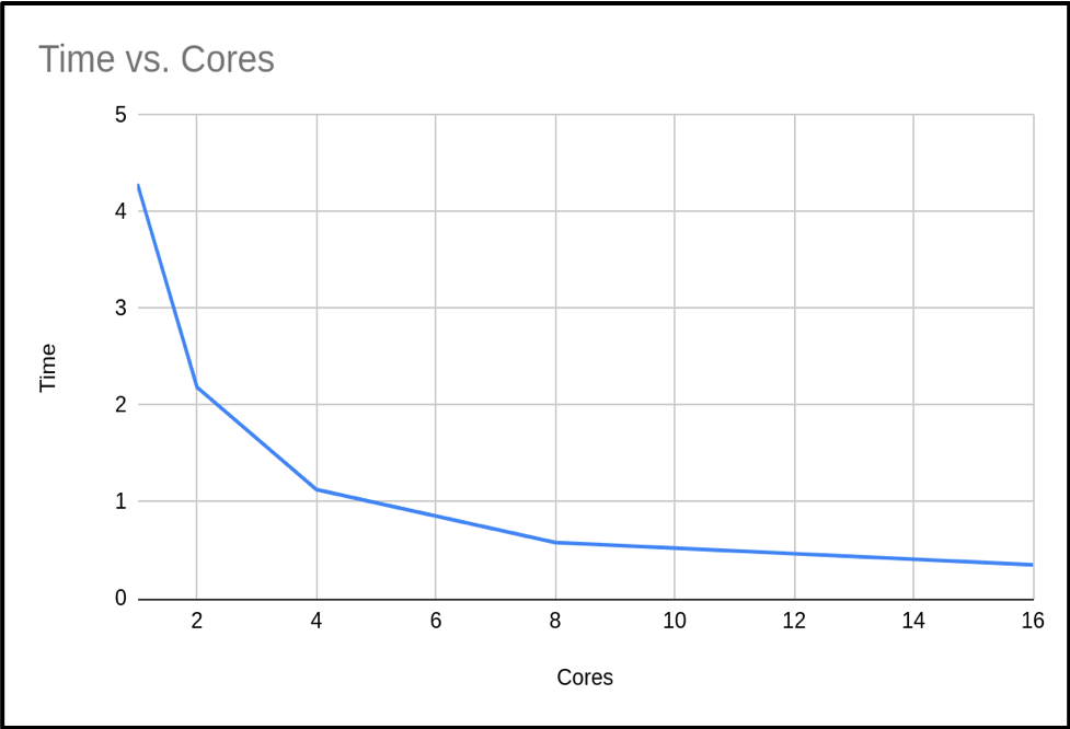
So we can see that as the number of cores increases, the run time of our program decreases. This makes sense, since we are splitting the calculation into smaller pieces which are executed at the same time.
Amdahl’s Law
If we use n processors, we might expect n times speedup. But as we’ve mentioned, this is rarely, if ever, the case! In a program, there is always some portion of it which must be executed in serial (such as initialisation routines, I/O operations and inter-communication) which cannot be parallelised. This limits how much a program can be speeded up, as the program will always take at least the length of the serial portion. This is actually known as Amdahl’s Law, which states that a program’s serial parts limit the potential speedup from parallelising the code.
We can think of a program as being operations which can and can’t be parallelised, i.e. the part of the code we can and can’t be speeded up. The time taken for a program to finish executing is the sum of the fractions of time spent in the serial and parallel portion of the code,
Time to Complete (T) = Fraction of time taken in Serial Portion (FS) + Fraction of time taken in Parallel Portion (FP)
T = FS + FP
When a program executes in parallel, the parallel portion of the code is split between the available cores. But since the serial portion is not split in this way, the time to complete is therefore,
Tn = FS + FP / n
We can see that as the number of cores in use increases, then the time to complete decreases until it approaches that of the serial portion. The speedup from using more cores is,
Speedup = T1 / Tn = ( FS + FP ) / ( FS + FP / n )
To simplify the above, we will define the single core execution time as a single unit of time, such that FS + FP = 1.
Speedup = 1 / ( FS + FP / n )
Again this shows us that as the number of cores increases, the serial portion of the code will dominate the run time as when n = ∞,
Max speedup = 1 / FS
What’s the Maximum Speedup?
From the previous section, we know the the maximum speedup achievable is limited to how long a program takes to execute in serial. If we know the portion of time spent in the serial and parallel code, we will theoretically know by how much we can accelerate our program. However, it’s not always simple to know the exact value of these fractions. But from Amdahl’s law, if we can measure the speedup as a function of number of cores, we can estimate that maximum speed up.
We can rearrange Amdahl’s law to estimate the parallel portion FP,
FP = n / ( n - 1 ) ( ( T1 - Tn ) / T1 )
Using the above formula on our example code we get the following results:
| Cores (n) | Tn | Fp | Fs = 1 - Fp |
|---|---|---|---|
| 1 | 3.99667 | - | - |
| 2 | 2.064242 | 0.967019 | 0.0329809 |
| 4 | 1.075068 | 0.974678 | 0.0253212 |
| 8 | 0.687097 | 0.946380 | 0.0536198 |
| 16 | 0.349366 | 0.973424 | 0.0265752 |
| Average | 0.965375 | 0.0346242 |
We now have an estimated percentage for our serial and parallel portion of our code. As you can see, as the number of cores we use increases, the time spent in the serial portion of the code increases.
Calculate using your Own Results II
Looking back at your own results from the previous Calculate using your Own Results I exercise, create new columns for Fp and Fs and calculate the results for each, using the formula above. Finally, calculate the average for each of these as in the table above.
Differences in Serial Timings
Similarly, in this instance we see that serial run times may vary depending on the run. There are several factors that are impacting our code. Firstly as we’ve discussed, these were run on a working system with other users, so runtime will be affected depending on the load of the system. Throughout DiRAC, it is normal when you run your code to have exclusive access, so this will be less of an issue. But if, for example, your code accesses bulk storage then there may be an impact since these are shared resources. As we are using the MPI library in our code, it would be expected that the serial portion will actually increase slightly with the number of cores due to additional MPI overheads. This will have a noticeable impact if you try scaling your code into the thousands of cores.
If we have several values, we can take the average to estimate an upper bound on how much benefit we will get from adding more processors. In our case then, the maximum speedup we can expect is,
Max speedup = 1 / FS = 1 / ( 1 - FP ) = 1 / ( 1 - 0.965375 ) = 29
Using this formula we can calculate a table of the expected maximum speedup for a given FP:
| FP | Max Speedup |
|---|---|
| 0.0 | 1.00 |
| 0.1 | 1.11 |
| 0.2 | 1.25 |
| 0.3 | 1.43 |
| 0.4 | 1.67 |
| 0.5 | 2.00 |
| 0.6 | 2.50 |
| 0.7 | 3.33 |
| 0.8 | 5.00 |
| 0.9 | 10.00 |
| 0.95 | 20.00 |
| 0.99 | 100.00 |
Number of Cores vs Expected Speedup
Using what we’ve learned about Amdahl’s Law and the average percentages of serial and parallel proportions of our example code we calculated earlier in the Calculate using your Own Results II exercise, fill in or create a table estimating the expected total speedup and change in speedup when doubling the number of cores, in a table like the following (with the number of cores doubling each time until a total of 4096). Substitute the initial T1
???????value with the initial Tn value from your own run.Hints: use the following formula:
Tn = Fs + ( Fp / n )
Speedup = T1 / Tn
Cores (n) Tn Speedup Change in Speedup 1 ??????? 2 4 … 4096 When does the change in speedup drop below 1%?
Solution
How closely do these estimations correlate with your actual results to 16 cores? They should hopefully be similar, since we’re working off averages for our serial and parallel proportions.
Hopefully from your results you will find that we can get close to the maximum speedup calculated earlier, but it requires ever more resources. From our own trial runs, we expect the speedup to drop below 1% at 4096 cores, but it is expected that we would never run this code at these core counts as it would be a waste of resources.
Using the
3.9967T1 starting value, we get the following estimations:
Cores (n) Tn Speedup Change in Speedup 1 3.99667 1 0 2 2.067504 1.933089 0.933089 4 1.102943 3.623642 1.690553 8 0.620662 6.439365 2.815723 16 0.379522 10.530804 4.091439 32 0.258952 15.434038 4.903234 64 0.198667 20.117475 4.683437 128 0.168524 23.715726 3.598251 256 0.153453 26.044951 2.329225 512 0.145917 27.389997 1.345046 1024 0.142149 28.115998 0.726001 2048 0.140265 28.493625 0.377627 4096 0.139323 28.686268 0.192643
How Many Cores Should we Use?
From the data you have just calculated, what do you think the maximum number of cores we should use with our code to balance reduced execution time versus efficient usage of compute resources.?
Solution
Within DiRAC we do not impose such a limit, this is a decision made by you. Every project has an allocation and it is up to you to decide what is efficient use of your allocation. In this case I personally would not waste my allocation on any runs over 128 cores.
Calculating a Weak Scaling Profile
Not all codes are suited to strong scaling. As seen in the previous example, even codes with as much as 96% parallelizable code will hit limits. Can we do something to enable moderately parallelizable codes to access the power of HPC systems? The answer is yes, and is demonstrated through weak scaling.
The problem with strong scaling is as we increase the number of cores, then the relative size of the parallel portion of our task reduces until it is negligible, and then we can not go any further. The solution is to increase the problem size as you increase the core count – this is Gustafson’s law. This method tries to keep the proportion of serial time and parallel time the same. We will not get the benefit of reduced time for our calculation, but we will have the benefit of processing more data. Below is a re-run of our π code. But this time, as we increase the cores we also increase the samples used to calculate π.
| Cores (n) | Run Time | Result | Error | % Improved Error |
|---|---|---|---|---|
| 1 | 4.149807 | 3.14159265459 | 0.00000003182 | |
| 2 | 4.362416 | 3.14159265409 | 0.00000001591 | 50.00% |
| 4 | 5.205988 | 3.14159265384 | 0.00000000795 | 75.02% |
| 8 | 4.356564 | 3.14159265371 | 0.00000000397 | 87.52% |
| 16 | 4.643724 | 3.14159265365 | 0.00000000198 | 93.78% |
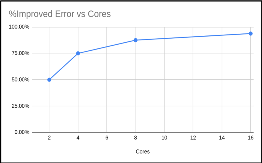
As you can see, the run times are similar. Just slightly increasing. However, the accuracy of the calculated value of π has increased. In fact our percentage improvement is nearly in step with the number of cores.
When presenting your weak scaling it is common to show how well it scales, this is shown below:
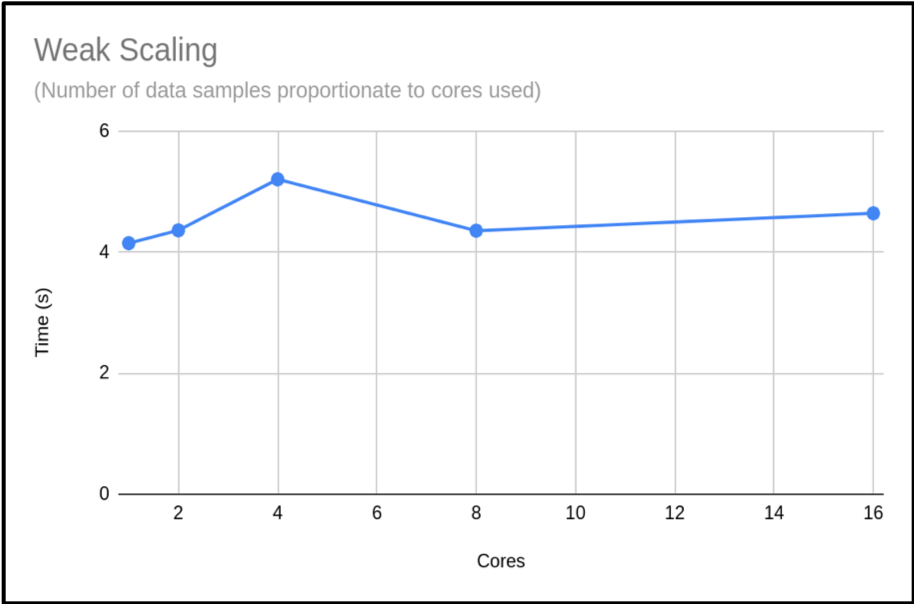
We can also plot the scaling factor. This is the percentage increase in run time compared to base run time for a normal run. In this case we are just using T1:

The above plot shows that the code is highly scalable. We do have an anomaly with our 4 core run, however. It would be good to rerun this to get a more representative sample, but this result is a common occurrence when using shared systems. In this example we only did a single run for each core count. When compiling your data for presentation or submitting applications, it would be better to do many runs and exclude outlying data samples or provide an uncertainty estimate.
Calculate using your Own Results III
You can reproduce this weak scaling profile with the Pi code by submitting a job which executes the following instead, in
mpi-pi.sh:... ./run.sh WeakBy passing this argument, our program is able to provide timings for a weak profile, scaling up the required accuracy for Pi accordingly. Make this amendment, and see how your results compare.
Maximum Cores to Use?
It would be hard to estimate the max cores we could use from this plot. Can you suggest an approach to get a clearer picture of this code’s weak scaling profile?
Solution
The obvious answer is to do more runs with higher core counts, and also try to resolve the n = 4 sample. This should give you a clearer picture of the weak scaling profile.
Obtaining Resources to Profile your Code
It may be difficult to profile your code if you do not have the resources at hand, but DiRAC can help. If you are in a position of wanting to use DiRACs facilities but do not have the resources to profile your code, then you can apply for a Seedcorn project. This is a short project with up to 100,000 core hours for you to profile and possibly improve your code before applying for a large allocation of time.
Key Points
We can use Amdahl’s Law to understand the expected speedup of a parallelised program against multiple cores.
It’s often difficult to estimate the proportion of serial code in our programs, but a reformulation of Amdahl’s Law can give us this based on multiple runs against a different number of cores.
Run timings for serial code can vary due to a number of factors such as overall system load and accessing shared resources such as bulk storage.
The Message Passing Interface (MPI) standard is a common way to parallelise code and is available on many platforms and HPC systems, including DiRAC.
When calculating a strong scaling profile, the additional benefit of adding cores decreases as the number of cores increases.
The limitation of strong scaling is the fixed problem size, and we can increase the problem size with the core count to obtain a weak scaling profile.
Survey
Overview
Teaching: min
Exercises: minQuestions
Objectives
Key Points