Landscape of HPC Technologies
Last updated on 2025-11-06 | Edit this page
Estimated time: 0 minutes
Overview
Questions
- Which programming language should I use?
- What are the main ways we can parallelise a program on modern HPC systems?
- How do OpenMP and MPI differ in how they achieve parallelism?
- What role do GPUs play in HPC, and how do approaches like CUDA and OpenACC use them?
Objectives
- Differentiate at a high level between the features of OpenMP, MPI, CUDA and OpenACC
- Briefly summarise the main OpenMP compiler directives and what they do
- Describe how to compile and run an OpenMP program
- Briefly summarise the main MPI message-passing features and how they are used
- Describe how to compile and run an MPI program
- Briefly summarise how an OpenACC program is written, compiled and run
- Briefly summarise how a CUDA program is written, compiled and run
To get the most performance possible, high-performance computing relies on parallelism. Modern systems combines tens of thousands of processors, each working on their own part of the problem. To be able to wield this power, we need to understand how to write parallel code. This is far more complicated than the scope of this episode. Therefore we will, instead, look at the landscape of the core HPC technologies used today in research. In particular, we will look at the following parallel frameworks: OpenMP, MPI, OpenACC and CUDA.
Common programming languages
Before we start, let’s look at what programming languages are used in HPC. In principle, any programming language can be used to write code which runs on an HPC cluster. In practise, however, there are some languages which are better suited to writing highly performant code. Interpreted languages, such as Python, are easy to develop in, but are much slower to execute than compiled languages, making them less suitable for computation-heavy applications. For this reason, compiled languages such as C, C++ and Fortran are some of the most common choices of programming language when writing high performance applications as they produce fast, optimised executables.
Python does, however, remain widely used in HPC, typically by performance-critical sections of code being written in compiled languages and accessed through a Python interface. Frameworks such as PyTorch, NumPy, SciPy and Numba all rely on underlying C, Fortran and/or CUDA to accelerate computation, while libraries such as mpi4py or multiprocessing make it possible for distributed parallelism directly in Python. Hybrid approaches like this have become more common because they combine Python’s ease of use with the speed of compiled code.
Other specialised languages and frameworks are also used in HPC, depending on the application area. CUDA and ROCm are employed for GPU programming, while newer languages such as Julia aim to combine ease of development with high performance. Domain-specific tools like MATLAB, and R also appear in HPC environments, though they often rely on compiled extensions or external libraries for parallel execution.
So which language should you use? There is no simple answer. The best choice depends heavily on your specific application, the target hardware (like CPUs or GPUs), and the trade-offs you are willing to make between raw computational performance and ease of development. Ultimately, the right language is the one that allows you to solve your problem efficiently, leveraging the available libraries and expertise within your team.
Which compiler should you use?
Iridis and most HPC systems offer a choice of compilers to use. But
which one should you use? In most cases, you would want to use the
compiler specific to the type of CPU you are using on the system,
because these implement architecture specific optimisations e.g. use
AMD’s aocc on Iridis 6. If you are using NVIDIA GPUs, you
have little choice in using anything other than NVIDIA’s
nvc, nvcc or nvfortran
compilers.
However, the code you are using may only have been tested on a specific compiler such as GCC. In those cases, it’s often best to stick with what is known to work. However, there is nothing stopping you using Intel’s compilers on an AMD based system, if the code is only tested or depends on features in the Intel compilers.
A simple example
We’ll now take a high level look at a selection of some of the most used libraries and frameworks used to parallelise code in research. In particular, we will see how to use them, the code changes required and how to run them on Iridis. The intention is not to make you proficient with these frameworks–or even dangerous–but to give a high level appreciation on what is being used.
To illustrate this, we will use a simple program, written in C, which
adds together two vectors to explore the code changes required. More
specifically, we will be modifying the following function
vector_add to run in parallel. We have chosen to use C as
it is commonly used language in HPC.
C
// *a, *b, and *c are arrays and n is the length of them.
// The result of the addition is returned back in *c
void vector_add(int *a, int *b, int *c, int n) {
    // This is the loop which we'll parallelise
    for (int i = 0; i < n; ++i) {
        c[i] = a[i] + b[i];
    }
}
You can find the entire program in vector_serial.c. To run this code on Iridis X, we’ll use the following submission script.
BASH
#!/bin/bash

#SBATCH --partition=amd
#SBATCH --nodes=1
#SBATCH --ntasks=1
#SBATCH --time=00:01:00

# Load the gcc module, which is the compiler we'll use
module load gcc

# Compile the program using gcc
gcc vector_serial.c -o vector_serial.exe

# Run the compiled executable
./vector_serial.exe
After the program has run, we should see the following output.
OUTPUT
Verification (first 5 elements):
c[0] =   0 (expected:   0)
c[1] =   3 (expected:   3)
c[2] =   6 (expected:   6)
c[3] =   9 (expected:   9)
c[4] =  12 (expected:  12)
OpenMP
The first framework we’ll look at is OpenMP. As mentioned in the previous episode, OpenMP is an industry-standard framework designed for parallel programming in a shared-memory environment. OpenMP spawns threads with each one, ideally, running on its own CPU core. OpenMP works by using compiler directives to tell the compiler which code needs to be parallelised, letting OpenMP and the compiler take care of all the low-level parallelisation details. In general, you just need to say which parts of your code you want to run in parallel.
Compiler directives
If you’re unfamiliar with compiler directives, you can think of them
as being a special command for the compiler, not for the
program itself. In C and C++, these almost always start with
#pragma. Think of it as a special note to the compiler
which says, “when you compile this specific piece of code, do something
extra.” Since these are compiler options, they do not modify the run
time behaviour of the program, only how the program is compiled.
Parallelisation with OpenMP is handled with these compiler
directives. However, OpenMP does also offer a library of runtime
functions which gives finer grained control, such as if you need to
ensure thread synchronisation or need to go off the beaten track. To
parallelise our vector_add function, we only need to add a
single line of code, using a compiler directive, just before the
loop.
C
void vector_add(int *a, int *b, int *c, int n) {
// This directive tells OpenMP to spawn threads and to
// divide the loop iterations between them. Each thread will
// handle a fraction of the loop iterations/vector addition
#pragma omp parallel for
    for (int i = 0; i < n; ++i) {
        c[i] = a[i] + b[i];
    }
}
The full program is in vector_openmp.c. Let’s break
this down more. The directive we used,
#pragma omp parallel for, tells the compiler that the next
for loop should be parallelised. The compiler then automatically
parallelises it for us, creating a team of threads and dividing the
loop’s work among them. In this case, each thread will perform a portion
of the vector addition. All OpenMP directives begin with
#pragma omp, followed by a specific command.
There are lots of other directives available, with
#pragma omp parallel for being the most commonly used.
Another useful directive is #pragma omp atomic which
prevents multiple threads from modifying a variable at once. This is one
way to prevent the race conditions mentioned in the previous episode.
OpenMP also provides a library of runtime functions which offers even
more control. For example, we can use the function
omp_set_num_threads() to control the number of threads that
OpenMP will spawn. In C, we need to include the appropriate header file,
<omp.h>, to access the library functions.
C
#include <omp.h>

void vector_add(int *a, int *b, int *c, int n) {
    // Manually set the number of threads to 8
    omp_set_num_threads(8);

#pragma omp parallel for
    for (int i = 0; i < n; ++i) {
        c[i] = a[i] + b[i];
    }
}Directives and functions for synchronisation
Effective control of thread synchronisation is essential when parallelising code with OpenMP, as improper handling of shared data can lead to race conditions and unpredictable results. To support this, OpenMP provides a range of directives and library functions that coordinate access to shared data and manage thread behaviour. The tables below summarise several commonly used examples.
| Compiler Directive | Description |
|---|---|
#pragma omp atomic |
Ensures a specific operation, such as modifying a variable, is executed atomically, e.g. by one thread at a time, to prevent race conditions. |
#pragma omp critical |
Defines a region of code that only one thread can execute at a time. |
This list is not exhaustive. A complete reference for all OpenMP directives and functions is available in the OpenMP 6.0 Reference Guide.
To compile an OpenMP program, we need to use the
-fopenmp flag,
e.g. gcc -fopenmp vector_openmp.c. If we don’t use the
-fopenmp flag, the compiler directives are ignored and any
library functions from <omp.h> will not be found
resulting in a compilation error.
Do I need to keep the serial version?
Setting the number of threads or processes to one will produce the
same behaviour as the serial program, assuming no programming errors.
However, to be extra safe, you can use conditional
compilation to maintain both parallel and serial versions within the
same codebase/file. Compiled languages support conditional compilation,
which allows certain sections of code to be compiled only if a specific
condition is met. When using OpenMP, the compiler variable
_OPENMP is defined when the -fopenmp flag is
passed, so you can use this variable to prevent OpenMP directives and
functions from being compiled when -fopenmp is not
used.
To launch an OpenMP program, run it like any other program. The
number of threads for OpenMP to use can be controlled using the
environment variable OMP_NUM_THREADS, or the
omp_set_num_threads() function discussed earlier. If the
function is unused and the environment variable left unset, OpenMP will
spawn one thread per CPU core. Normally, on a HPC cluster this is
probably what is wanted. However, when running on your own computer
during development and testing, you will probably want to set
OMP_NUM_THREADS to be less than then number of CPU cores to
avoid overloading your computer.
The following is an example of how you would compile and launch an OpenMP program on Iridis X, in a single submission script.
BASH
#!/bin/bash

#SBATCH --partition=amd
#SBATCH --nodes=1
#SBATCH --ntasks=1
#SBATCH --cpus-per-task=8
#SBATCH --time=00:01:00

# Use OMP_NUM_THREADS to say we can to use --cpus-per-task number of
# threads. The --cpu-per-task SBATCH directive is populated into the
# SLURM_CPUS_PER_TASK environment variable
export OMP_NUM_THREADS=$SLURM_CPUS_PER_TASK

# Compile the program using gcc
module load gcc
gcc -fopenmp vector_openmp.c -o vector_openmp.exe

# We run the compiled executable just like the serial version
./vector_openmp.exe
The main advantage of OpenMP is that it requires only minimal code modification to parallelise existing programs, particularly when the main computational workload lies within loops. Beyond simple loop-level parallelism, parallelising more complex program structures becomes more challenging, though this is true of most parallel frameworks. OpenMP still provides a wide range of straightforward directives, making it easy to adapt serial code without needing to design the program for parallel execution from the start. Its main limitation is that it uses a shared-memory model, which requires careful management of thread synchronisation and restricts scalability to a single compute node.
Message Passing Interface (MPI)
The Message Passing Interface (MPI) was designed to enable scientific applications to run on supercomputers and, as such, has become the dominant distributed-memory parallelism framework in research. An MPI application creates many processes each working on their own individual task. However, unlike shared-memory approaches, each MPI process–or rank–has its own private memory space. Therefore to exchange data between these ranks, explicit communication has to happen. This is where MPI comes in. It provides a set of library functions to configure a parallel environment and exchange data within it. The key concept in MPI is message passing, which involves the explicit exchange of data between processes. Processes can send messages to specific destinations, broadcast messages to all processes, or perform collective operations where all processes participate.
To achieve parallelism, each process runs a copy of the same program as the other processes, but works on its own subset of data, or does its own tasks. The processes communicate to exchange data and/or coordinate their next tasks. The power of MPI is that the processes can run on different nodes, allowing MPI programs to scale well beyond a single machine. Thankfully the complexity of having to spawn processes on different nodes and communicate over the network is hidden away and controlled by MPI’s library of functions and the HPC cluster’s scheduler/resource manager, e.g. Slurm on Iridis.
But there are some trade-offs with MPI. In terms of performance, communicating data takes time. If you have a method which requires frequent communication or data dependencies, then you will spend more time exchanging data than doing computation. It may instead be worth using a shared-memory framework like OpenMP. However the biggest trade-off, by far, is that you need to design your application in mind for MPI parallelisation. Unlike OpenMP, it is not simple to retrofit a serial program with MPI. For example, we need to make sure we program initialising the MPI library ourselves, track process IDs, explicitly send and receive data, coordinate the processes so they do their own work, and so on. The table below gives an idea of some of the MPI functions we need to use and their purpose.
| Function | Description |
|---|---|
MPI_Init |
Initialises the MPI environment. Must be called before any other MPI calls. |
MPI_Comm_size |
Returns the total number of processes in the communicator. |
MPI_Comm_rank |
Returns the rank (ID) of the calling process. |
MPI_Send / MPI_Recv
|
Used for direct point-to-point communication between processes. |
MPI_Barrier |
Used for synchronisation. A processes cannot continue past the barrier until all processes have reached it. |
MPI_Finalize |
Shuts down the MPI environment. Must be called before exiting the program, other wise background MPI tasks may not finish. |
This is only a tiny glimpse into the available MPI functions, and what you can do with MPI. In total, there are around 500 functions.
Let’s now take a look at the code changes we need to parallelise the
add_vector function using MPI. A detailed description of
the MPI library functions, and how to design an MPI program, is out of
scope for this episode, and lesson, so we won’t go much into the
details. From a high level, what we need to do is: 1) initialise the MPI
environment, 2) split the work between processes, 3) have each process
do their work, and 4) communicate the results back to one or more
processes for the cycle to repeat. The example code below demonstrates
this. Keep in your head that each process is executes the
exact same function, but will do something different
based on its ID.
C
//Include the MPI header file to access the MPI functions
#include <mpi.h>

void vector_add(int *a, int *b, int *c, int n) {
    // Initialise the MPI environment -- nothing will work if we
    // don't do this
    MPI_Init(NULL, NULL);

    // Get the rank (process ID) and total number of processes launched
    int rank, size;
    int root_rank = 0;
    MPI_Comm_rank(MPI_COMM_WORLD, &rank);
    MPI_Comm_size(MPI_COMM_WORLD, &size);

    // Determine next how many elements of the vector this process
    // will handle. We will create a "local" array which will store
    // the results of the vector addition for this process
    int n_local = n / size;
    int c_local[n_local];

    // Determine the subset of the vectors a and b this process
    // will be adding together. To do this, we use the ID of
    // the process and the number of elements each process
    // will be working on
    int start = rank * n_local;
    int stop = (rank + 1) * n_local;

    // Perform the local computation on each process
    for (int i = start; i < stop; i++) {
        c_local[i] = a[i] + b[i];
    }

    // We can use this MPI_Gather function to send the "partial" results
    // from each process back to the "root" process. Only the root process
    // will have the complete vector
    MPI_Gather(c_local, n_local, MPI_INT, c, n_local, MPI_INT,
               root_rank, MPI_COMM_WORLD);

    // Finalise the MPI environment
    MPI_Finalize();
}
The complete program is in vector_mpi.c. As you can see, the code is much more involved than the OpenMP example. Every process runs this same function, but each one is responsible for a different part of the vector addition. Each process follows a clear set of steps:
- First, it finds out its unique ID (
rank) and the total number of processes (size). - Using this, it calculates which “slice” of the vectors
aandbit is responsible for. - It then performs the addition for its slice and stores the partial
answer in a local
c_localarray. - Finally, it calls the
MPI_Gatherfunction, which aggregates all thec_localarrays.
MPI_Gather is a collective communication shortcut.
Behind the curtain it doing the MPI_Send and
MPI_Recv for us, sending data from each process back to our
root process; which is the only process with the complete result.
Challenge
Why does only the “root” process have the final, complete, result?
It is because we used MPI_Gather to “gather” the results
from each process back to the root process. There is no communication to
the other process, so only the root process has the data from the other
processes. If we wanted every process to have a copy of the final result
of c, we could instead use MPI_Allgather.
To compile an MPI application, we need to use an MPI-aware
compiler which is essentially a clever script which knows where MPI is
installed on our system to make compilation easier. On Iridis, this is
mpicc. We use mpicc as we would any other
compiler: mpicc vector_mpi.c -o vector_mpi.exe.
What’s an MPI-aware compiler?
An MPI-aware compiler is essentially a script which wraps around your
regular compiler to provide the required header files and libraries to
the compiler to build an MPI application. In theory, we could find those
headers and libraries ourselves and pass them the compiler instead.
However, in practise, this is not worth our time when mpicc
already does it for us.
To launch an MPI application we need to use mpirun,
e.g. mpirun vector_mpi.exe. This is another script provided
by MPI which handles launching the parallel processes and setting up the
parallel environment. If we run the program without using
mpirun, then only a single processes will start and will
probably become “deadlocked” as the program waits indefinitely for
messages from other processes that were never sent. On Iridis, and other
Slurm clusters, we can alternatively use the Slurm launcher
srun to do the same job. To summarise, the purposes of
srun and mpirun is to,
- Read the environment to see how many processes to create (e.g., from
#SBATCH --ntasks=8). - Launch that many copies of your executable.
- Manage where these processes run. If you request resources across multiple nodes, the launcher (in coordination with Slurm) starts the processes on the correct machines and ensures they can all communicate with each other.
The following is an example of how you would compile and launch an MPI program on Iridis X.
BASH
#!/bin/bash

#SBATCH --partition=amd
#SBATCH --nodes=1
#SBATCH --ntasks=8
#SBATCH --cpus-per-task=1
#SBATCH --time=00:01:00

# Load the specific MPI library we want to use
# This makes the 'mpicc' and 'mpirun' commands available
module load openmpi

# Compile the code using the MPI compiler wrapper
mpicc vector_mpi.c -o vector_mpi.exe

# Launch the program using 'srun'. This is the recommended
# launcher on Slurm clusters. 'srun' automatically reads the
# SBATCH settings and launches 8 (from --ntasks) copies
# of our executable
srun ./vector_mpi.exe

# -----------------------------------------------------------
# An alternative way to launch the program
# 'mpirun' is the more traditional MPI launcher. Here, we
# must explicitly tell it how many processes (-np) to run
# We use the $SLURM_NTASKS variable (which Slurm sets to 8)
# to match our resource request
# mpirun -np $SLURM_NTASKS ./vector_mpi.exe
# -----------------------------------------------------------Hybrid MPI+OpenMP
MPI and OpenMP don’t have to be competing choices. They can be used together in a hybrid parallel model, where MPI distributes work across nodes and OpenMP manages threads within each node. This combination allows applications to scale beyond a single machine while using memory and CPU cores more efficiently.
Hybrid parallelism reduces data duplication between processes and improves load balancing through OpenMP’s flexible scheduling. It also helps lower communication costs by keeping shared-memory operations local to a node.
The main drawbacks are added complexity and potential overheads from managing both models. Code becomes harder to write, debug, and port between systems. Still, hybrid MPI+OpenMP programs are often the best solution for large-scale workloads where pure MPI or OpenMP alone falls short.
Challenge
Why does using a hybrid MPI+OpenMP scheme reduce data duplication?
In a pure MPI application, you would run many separate processes on a single compute node (e.g., 64 processes on 64 cores). Each MPI process has its own private memory. If all 64 processes need to access the same 10GB input file, that 10GB of data must be loaded 64 times, once into each process’s memory. This duplicates the data 64 times, using 640GB of RAM on that node just for that one file.
In a hybrid MPI+OpenMP model, you may run only one MPI process on that node. That single process would then use OpenMP to spawn 64 threads, one for each core. Because all OpenMP threads share the memory of their parent process, the 10GB input file only needs to be loaded once. All 64 threads can access that single copy, reducing the memory footprint for that data from 640GB to just 10GB.
Using GPUs instead of CPUs
Besides using multiple CPUs, we can also use Graphical Processing Units (GPUs) to do calculations in parallel. GPUs were originally designed to speed up rendering to display images to a screen, a task that involves performing millions of simple, repetitive calculations in parallel. Researchers soon realised this design was also perfect for many scientific problems.
GPUs are highly parallel, built to perform thousands of operations at the same time. This makes them ideal for work that can be split into many identical, independent tasks. While CPUs are designed to tackle complex tasks one after another, GPUs are optimised for doing the exact same operation on large amounts of data simultaneously. This is perfect for problems like matrix operations, where every element can be processed in the same way.
However, offloading work to a GPU is more complicated than parallelising using CPUs. The main reason is that the CPU and the GPU have their own separate memory spaces. Data stored in the CPU’s memory is not visible to the GPU, and vice-versa. This setup is similar to the separate memory for each process in an MPI application. Data must be copied from the CPU’s memory to the GPU’s memory. This transfer step is slow compared to the speed of the calculations. Therefore, efficient GPU programs must minimise data transfers, often by keeping data on the GPU as long as possible. While optimising CPU code often focuses on reducing the total number of calculations, optimising GPU code is usually more about reducing data transfers and organising data efficiently in the GPU’s memory.
This level of detail is beyond the scope of this introduction. As before, we will only give a broad overview of two popular frameworks: OpenACC and CUDA. You can think of these as being similar to OpenMP and MPI:
- OpenACC is like OpenMP: you can often add it to existing code, using compiler directives to automatically handle the parallelisation.
- CUDA is “similar” to MPI: it is a more complex framework that requires you to design your program around it.
CPU and GPU, what’s the difference?
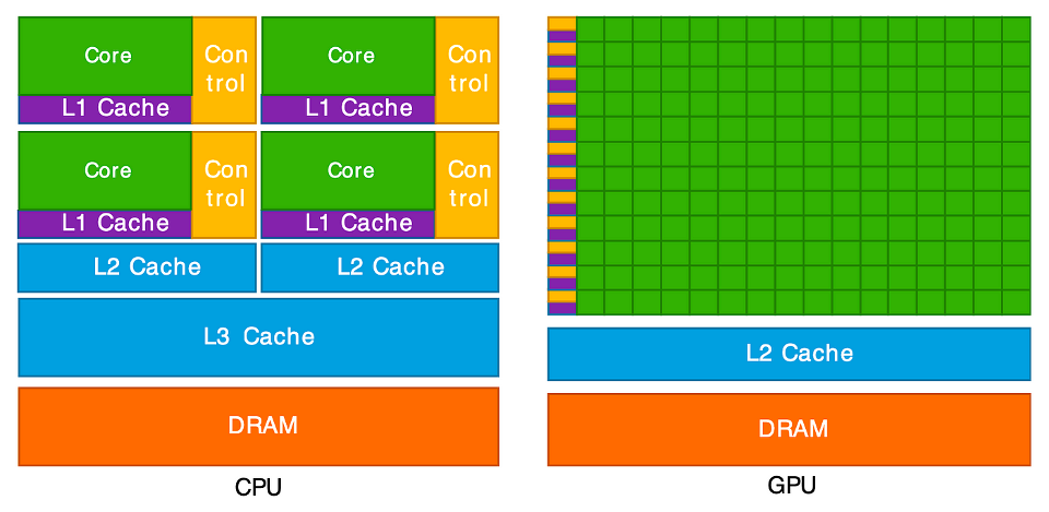
This diagram illustrates the key difference between a CPU and a GPU. On the left, the CPU is shown with a few, large “Cores” (green). Each core is complex, paired with significant “Control” logic (yellow) and large, fast memory caches (purple and blue). This design makes each CPU core very “smart” and powerful, ideal for handling complex instructions and varied tasks one after another.
On the right, the GPU has a completely different structure. It is
composed of hundreds or even thousands of tiny, simple cores (the large
green grid). Notice how much less space is dedicated to “Control” logic
and complex caches. This architecture is not designed for complex,
sequential tasks. Instead, it is a massive parallel workforce, built to
execute the same simple operation (like c[i] = a[i] + b[i])
at the same time across thousands of different pieces of data. This
“many-core” design is what allows it to perform thousands of operations
concurrently.
GPUs also use a different memory model. Each GPU core can access the large global memory, which is shared across the entire GPU. It is slower to read and write to this. To improve performance, groups of cores are organised into blocks which shared a small, but very fast, memory area. This setup is similar to shared-memory parallelism on CPUs, where threads cooperate through a common memory space. However, each GPU block’s shared memory is private to that block, much like how separate processes in a distributed-memory model (such as MPI) each have their own memory and must explicitly exchange data. Efficient GPU programs manage this hierarchy carefully, reusing shared memory to reduce costly access to global memory.
OpenACC
OpenACC is a framework for parallel programming on GPUs, both for NVIDIA and AMD GPUs; i.e. it is platform agnostic. Just like OpenMP, it uses compiler directives to tell the compiler which parts of code should be executed in parallel on a GPU. Also like OpenMP, the OpenACC runtime and compiler handles all of the parallelisation details such as generating the parallel code, transferring data between the CPU and GPU and synchronising/managing GPU threads.
Whilst most of the heavy lifting for OpenACC is done with compiler
directives, a runtime library is also available for finer control over
things such as selecting which GPU to use (if you are lucky enough to
have more than one!), finer grained data movement and synchronisation
mechanisms. To parallelise our vector_add function to a
GPU, we only need to add a single line of code.
C
void vector_add(int *a, int *b, int *c, int n) {
// This OpenACC directive tells the compiler to parallelise the
// following 'for' loop, running its iterations concurrently
// on the GPU
#pragma acc parallel loop
    for (int i = 0; i < n; ++i) {
        c[i] = a[i] + b[i];
    }
}
The full program is in vector_openacc.c. The directive
#pragma acc parallel loop tells the compiler to parallelise
the loop and execute it on the GPU. Each GPU core/thread performs part
of the vector addition. OpenACC also takes care of allocating memory on
the GPU and transferring data from the CPU to GPU’s memory. It also
copies the results back to the CPU when the loop is completed.
Some other useful directives
As we’ve seen,#pragma acc parallel loop targets a single
loop. OpenACC also provides the #pragma acc kernels
directive. This directive is meant to be put before a larger region of
code, such as a complicated loop or multiple loops. The compiler then
analyses this entire region and automatically determines the best way to
convert the code, including any loops it finds, into parallel “kernels”
of code to run on the GPU.
The main difference is that #pragma acc parallel loop is
prescriptive: you are explicitly telling the compiler to parallelise
that one loop. In contrast, #pragma acc kernels is
descriptive: you are telling the compiler “here is a block of code to
accelerate,” giving it freedom to analyse the code and choose the most
efficient way to parallelise and run it.
Additionally, whilst OpenACC automatically manages data transfers
between the GPU and CPU, more explicit data management is possible using
directives such as #pragma acc data, copy,
copyin, and copyout for more control.
To compile an OpenACC program, we need a compiler that supports it.
On Iridis X this is either GCC or one from NVIDIA’s compiler collection.
With GCC we need to use the -fopenacc flag. However, when
using NVIDIA’s C compiler, nvc, the flag is instead
-acc, e.g. nvc -acc vector_openacc.c. Without
the flag, the OpenACC directives are ignored and GPU code is not
generated.
The following is an example of how you would compile and launch an
OpenACC program on Iridis X. It is especially important that we remember
to request a GPU using the --gres=gpu:1 directive and
select a partition where nodes have GPUs.
BASH
#!/bin/bash

#SBATCH --partition=l4
#SBATCH --nodes=1
#SBATCH --ntasks=1
#SBATCH --cpus-per-task=1
#SBATCH --gres=gpu:1
#SBATCH --time=00:01:00

# Load the NVIDIA HPC SDK module, which provides OpenACC support
module load nvhpc

# Compile the program with GPU offloading enabled
nvc -acc vector_openacc.c -o vector_openacc.exe

# Check GPU availability and run the program
nvidia-smi
./vector_openacc.exe
The main advantage of OpenACC, like OpenMP, is that it allows rapid GPU parallelisation with minimal code changes. It is particularly useful for incrementally porting existing CPU applications to GPUs. However, compared to lower-level frameworks like CUDA, it offers less fine-grained control over GPU execution and memory management. OpenACC is therefore well suited for scientific and engineering applications where productivity are more important than maximal performance.
CUDA
The final framework we will look at is CUDA, which is essentially a programming language created by NVIDIA to run arbitrary code on NVIDIA GPUs. However, unlike OpenACC which uses compiler directives to automatically parallalise sections of code, CUDA is an extension of the C/C++ language which gives you explicit fine-grained control over the GPU. This is a much more powerful and performant approach, but also far more complex. You are no longer advising the compiler; you are directly writing the code that will run on the GPU. Given this complexity, we will only examine the key concepts at a very high level.
In CUDA, you write special functions called kernels that are
executed on the GPU. In the later code example below, we have two
functions: vector_add_kernel and vector_add.
The vector_add_kernel function is the code which runs on
the GPU. The __global__ keyword tells the compiler that
this function should be launched from the CPU but run on the GPU. Inside
this kernel, each thread calculates its own unique ID using special
variables (like blockIdx.x and threadIdx.x).
This ID determines which element i of the vector
c that specific thread will process. This is the core
mechanism for dividing the parallel work. You will also see an
if (i < n) check in the kernel. This is a crucial safety
check. GPUs launch threads in fixed-size groups, so you often launch
more threads than you have data (e.g., launching 1024 threads for a
1000-element array). This if statement simply tells the
“extra” threads (1000, 1001, etc.) to do nothing. Without it, they would
try to access memory that doesn’t exist, which could corrupt your data
or crash the program.
The original vector_add functions runs on the CPU and
manages the GPU, controlling when the GPU kernel is launched. It must
now do all the work manually that OpenACC handled
automatically:
- Allocate Memory:
cudaMallocis used to allocate separate memory for the three vectors (d_a,d_b,d_c) on the GPU’s memory. Thed_prefix is a common convention to mean “device” memory. - Copy Data In:
cudaMemcpy(withcudaMemcpyHostToDevice) is called to copy the input data from the CPU’saandbarrays to the GPU’sd_aandd_barrays. This is the explicit data transfer. - Launch Kernel: The
<<<grid, BLOCK_SIZE>>>syntax is the CUDA-specific command to launch the kernel. This tells the GPU to launch a “grid” of “blocks,” to execute thevector_add_kernelfunction. - Copy Data Out: After the kernel finishes,
cudaMemcpy(withcudaMemcpyDeviceToHost) copies the result from the GPU’sd_carray back to the CPU’scarray. - Clean Up:
cudaFreereleases the memory on the GPU.
CPP
// This is the "kernel" - the code that runs on the GPU a.k.a. the device
__global__ void vector_add_kernel(int *a, int *b, int *c, int n) {
    // Calculate the unique ID for this thread
    int i = blockIdx.x * blockDim.x + threadIdx.x;

    // Ensure the thread ID is within the bounds of the array
    if (i < n) {
        c[i] = a[i] + b[i];
    }
}

// This is the "host" function - the code that runs on the CPU
void vector_add(int *a, int *b, int *c, int n) {
    // Pointers for the "device" (GPU) memory
    int *d_a, *d_b, *d_c;
    int size = n * sizeof(int);

    // 1. Allocate memory on the GPU
    cudaMalloc(&d_a, size);
    cudaMalloc(&d_b, size);
    cudaMalloc(&d_c, size);

    // 2. Copy input data from CPU (host) to GPU (device)
    cudaMemcpy(d_a, a, size, cudaMemcpyHostToDevice);
    cudaMemcpy(d_b, b, size, cudaMemcpyHostToDevice);

    // 3. Launch the kernel on the GPU
    int BLOCK_SIZE = 256;
    int grid = (n + BLOCK_SIZE - 1) / BLOCK_SIZE;
    vector_add_kernel<<<grid, BLOCK_SIZE>>>(d_a, d_b, d_c, n);

    // 4. Copy the result from GPU (device) back to CPU (host)
    cudaMemcpy(c, d_c, size, cudaMemcpyDeviceToHost);

    // 5. Free the memory on the GPU
    cudaFree(d_a);
    cudaFree(d_b);
    cudaFree(d_c);
}
The full program is in vector_cuda.cu. To compile CUDA
code, we must use NVIDIA’s nvcc compiler. Note that this is
different from the nvc compiler we used to build the
OpenACC version of vector_add. The nvcc
compiler understands the CUDA-specific syntax used to define and launch
kernels, e.g. __global__ and
<<<...>>>. It separates out the
GPU-specific and CPU-specific code, compiling the CPU code using a
standard C++ compiler. CUDA files typically use the .cu extension.
To run a CUDA program, it is launched like any other program, as the mechanics to communicate and launch threads on the GPU is handled inside the program itself. The submission script for a CUDA code is nearly identical to the OpenACC script from before.
BASH
# !/bin.bash
# SBATCH --partition=a100
# SBATCH --nodes=1
# SBATCH --ntasks=1
# SBATCH --gres=gpu:1
# SBATCH --time=00:01:00

# Load the NVIDIA CUDA toolkit module
module load cuda

# Compile the program using nvcc
nvcc vector_cuda.cu -o vector_cuda.exe

# Run the executable (no special launcher needed)
./vector_cuda.exe
The main benefit of CUDA is the total control it provides, which often leads to the highest possible performance. The main drawbacks are its complexity (requiring manual memory management and kernel writing) and vendor lock-in, as CUDA code will only run on NVIDIA GPUs.
- Any language can be used for HPC, however, compiled languages like C, C++ and Fortran are typically used for performance-critical code. Python is often used on HPC using libraries which are built on compiled languages.
- OpenMP is a shared-memory model, using compiler directives
(
#pragma omp) to easily parallelise code (often loops) to run on the CPU cores of a single node. - MPI is a distributed-memory model, using a library of functions
(
MPI_Init,MPI_Send, etc.) to manage explicit communication between processes. It is complex but can scale across many nodes. - GPUs are “many-core” processors ideal for massive, simple, parallel tasks (like matrix maths). Using them requires copying data between the CPU (host) and GPU (device).
- OpenACC uses compiler directives (
#pragma acc) to offload work to a GPU, automating parallelisation and data transfers. - CUDA is a complex, explicit programming model for NVIDIA GPUs. It
requires you to write “kernels” and manually manage memory
(
cudaMalloc,cudaMemcpy) but offers the highest control and performance.