All Images
Introduction to HPC Systems
Figure 1

Iridis 6: One of Southampton’s High Performance
Computing clusters
Figure 2

Figure 3

Outsourcing Computational Tasks: many of the
tasks we perform daily using computers are outsourced to remote
servers
Figure 4
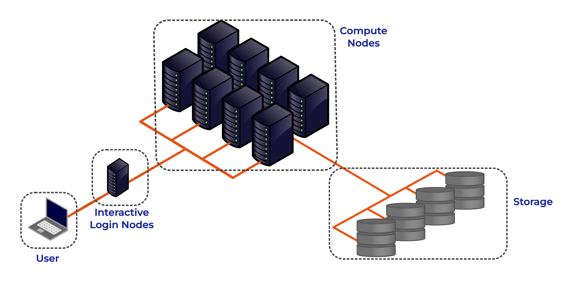
High Performance Computing System Architecture:
Simplified schematic of an HPC cluster.
Figure 5

High Performance Computing Landscape: In the UK
HPC facilities are divided into tiers based upon their size.
Figure 6

Figure 7

Figure 8

Figure 9

Figure 10

Figure 11

Figure 12

Figure 13

Figure 14

Figure 15

Figure 16

Figure 17
Figure 18

Accessing and Using HPC Resources
Figure 1
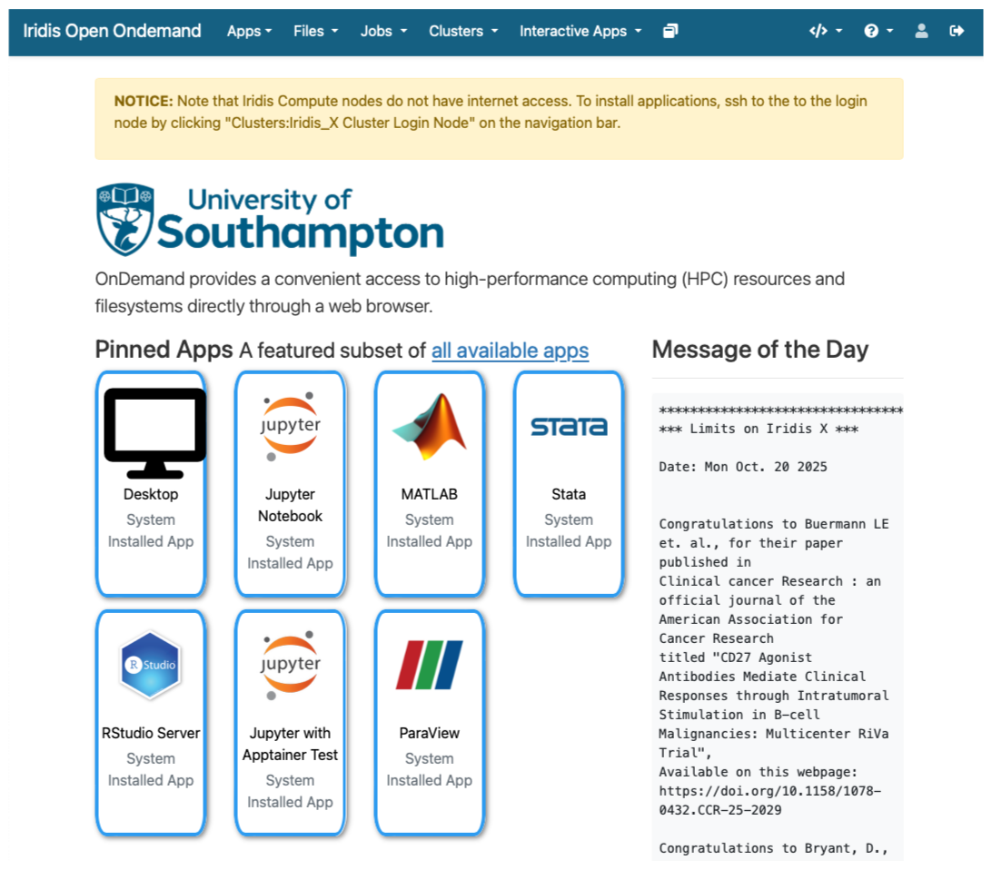
Iridis On Demand: A web portal to the University
of Southampton’s HPC Cluster, Iridis
Figure 2
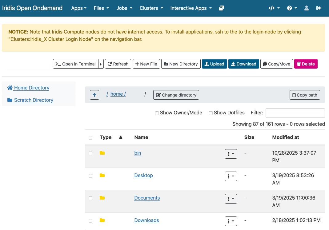
File Manager in Iridis On Demand: Moving data to
and from the Iridis HPC system can be achieved in the Open On Demand Web
Portal
Introduction to Job Scheduling
Figure 1

Queueing up to eat at a popular restaurant is
like queueing up to run something on an HPC cluster.
Introduction to Programmatic Parallelism
Figure 1
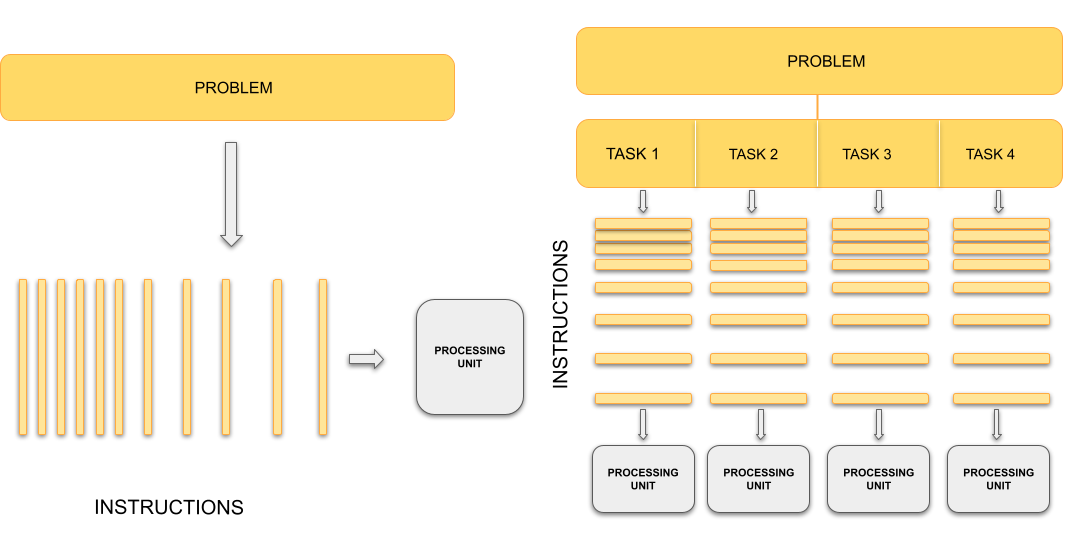
On the left, a single processing unit executes
one sequence of instructions for the whole problem. On the right, the
problem is divided into independent tasks, each processed concurrently
by separate processing units.
Figure 2

Multiple independent processes, each with their
own private memory space, communicating through explicit message passing
over a network.
Figure 3

Multiple threads within a single process,
sharing the same memory space and resources.
Figure 4
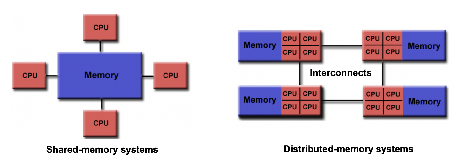
Comparison of shared and distributed memory
architectures: shared memory shows multiple processors accessing one
memory pool, while distributed memory shows processors each with private
memory connected by communication links.
Landscape of HPC Technologies
Figure 1
Measuring and improving parallel performance
Figure 1
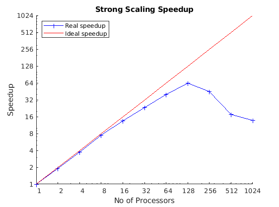
A plot showing the measured speed up against
number of processors. In this example, we can see that our code scales
very well up to 16 processors. However, beyond this amount the speed up
starts to diverge from ideal scaling. Once we start using 128 processors
we can see that it’s detrimental and the code performs worse!
Figure 2
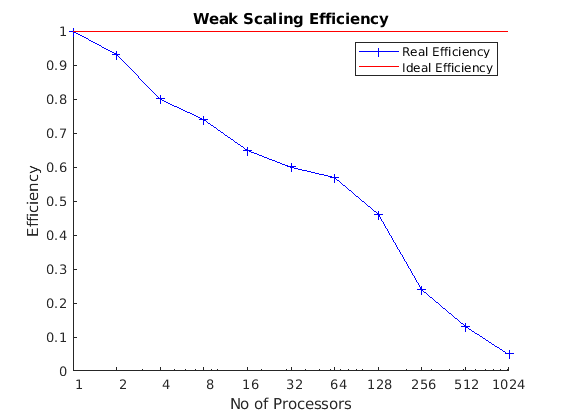
A plot showing the measured efficiency against
process count. We can see in this case that this code does not scale
well at all in a weak scaling test.