All in One View
Content from Introduction to HPC Systems
Last updated on 2025-11-04 | Edit this page
Estimated time: 0 minutes
Overview
Questions
- What is a High Performance Computing cluster?
- What is the difference between an HPC cluster and the cloud?
- How can an HPC cluster help me with my research?
- What HPC clusters are available to me and how do I get access to them?
Objectives
- Describe the purpose of an HPC system and what it does
- List the benefits of using an HPC system
- Identify how an HPC system could benefit you
- Summarise the typical arrangement of an HPC system’s components
- Differentiate between characteristics and features of HPC and cloud-based systems
- Summarise the capabilities of the NOCS HPC facilities
- Summarise the key capabilities of Iridis 6 and Iridis X for NOCS applications
- Summarise key capabilities of national HPC resources and how to access them
High Performance Computing

High Performance Computing (HPC) refers to the use of powerful computers and programming techniques to solve computationally intensive tasks. An HPC cluster, or supercomputer, is one which harnesses the aggregated power of groups of advanced computing systems. These high performance computers are grouped together in a network as a unified system, hence the name cluster. HPC clusters provide extremely high computational capabilities, significantly surpasssing that of a general personal computer.
Can you think of any computational research problems that could benefit from the aggregated computational power of High Performance Computing? Discuss it with your colleagues.
Here are some computation research examples where HPC could be of benefit: - A oceanography research student is modelling ocean circulation by processing seismic reflection datasets. They have thousands of these datasets - but each processing run takes an hour. Running the model on a laptop will take over a month! In this research problem, final results are calculated after all 1000 models have run, but typically only one model is run at a time (in serial) on the laptop. Since each of the 1000 runs is independent of all others, and given enough computers, it’s theoretically possible to run them all at once (in parallel).
The seismic reflection datasets are extremely large and the researcher is already finding it challenging to process the datasets on their computer. The researcher has just received datasets that are 10 times as large - analysing these larger datasets will certainly crash their computer. In this research problem, the calculations required might be impossible to speed up by adding more computers, but a computer with more memory would be required to analyse the much larger future data set.
An ocean modeller is using a numerical modelling system such as NEMO that supports parallel computation. While this option has not been used previously, moving from 2D to fully 3D ocean simulations has significantly increased the run time. In such models, calculations within each ocean subdomain are largely independent, allowing them to be solved simultaneously across processors while exchanging boundary information between adjacent regions. Because 3D simulations involve far more data and calculations, distributing the workload across multiple processors or computers connected via a shared network can substantially reduce runtime and make large-scale ocean simulations practical.
HPC clusters fundamentally perform simple numerical computations, but on an extremely large scale. In our examples we can see where HPC clusters excel, using hundreds or thousands of processors to complete a numerical task that would take a desktop or laptop days, months or years to complete. They can also tackle problems that are too large or complex for a PC to fit in their memory, such as modelling the ocean dynamics or the Earth’s climate.
High Performance Computing allows you as researchers to scale up your computational research and data processing, enabling you to do more research or to solve problems that would be infeasible to solve on your own computer.
HPC vs PC
Before we discuss High Performance Computing clusters in more detail let’s start with a computational resource we are all familiar with, the PC:
PC

|
Your PC is your local computing resource, good for small computational tasks. It is flexible, easy to set-up and configure for new tasks, though it has limited computational resources. Let’s dissect what resources programs running on a laptop require:
|
If Our PC isnt Powerful Enough?

When the task to solve becomes too computationally heavy, the operations can be out-sourced from your local laptop or desktop to elsewhere.
Take for example the task to find the directions for your next conference. The capabilities of your laptop are typically not enough to calculate that route in real time, so you use a website, which in turn runs on a computer that is almost always a machine that is not in the same room as you are. Such a remote machine is generically called a server.
The internet made it possible for these data centers to be far remote from your laptop. The server itself has no direct display or input methods attached to it. But most importantly, it has much more storage, memory and compute capacity than your laptop will ever have. However, you still need a local device (laptop, workstation, mobile phone or tablet) to interact with this remote machine.
There is a direct parallel between this and running computational workloads on HPC clusters, in that you outsource computational tasks to a remote computer.
However there is a distinct difference between the “cloud” and an HPC cluster. What people call the cloud is mostly a web-service where you can rent such servers by providing your credit card details and by clicking together the specs of a remote resource. The cloud is a generic term commonly used to refer to remote computing resources of any kind – that is, any computers that you use but are not right in front of you. Cloud can refer to machines serving websites, providing shared storage, providing web services (such as e-mail or social media platforms), as well as more traditional “compute” resources.
HPC systems are more static and rigidly structured than cloud systems, and follow consistent patterns in how they’re deployed, whereas cloud infrastructures tend to be much more flexible and “user-led” in their configurations and provisioning.
HPC Cluster
If the computational task or analysis is too large or complex for a single server, larger agglomerations of servers are used. These HPC systems are known as supercomputers, or described as HPC clusters as they are made up of a cluster of computers, or compute nodes.
Distinct to the cloud, these clusters are networked together and share a common purpose to solve tasks that might otherwise be too big for any one computer. Each individual compute node is typically a lot more powerful than any PC - i.e. more memory, many more and faster CPU cores. However in parallel to the cloud you access HPC clusters remotely, through the internet.
The figure below shows the basic architecture of an HPC cluster.
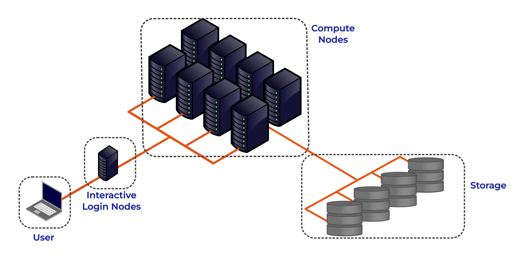
Lets go through each part of the figure:
Interactive Login Nodes
When you are given an account on an HPC cluster you will get some login credentials. Using these credentials you can remotely log-on to of the interactive login nodes from your local PC over the internet. There may be several login nodes, to make sure that all the users are not trying to access one single machine at the same time.
Once you have logged onto the login node you can now run HPC workloads, or jobs, on the HPC cluster. BUT you typically do not directly access the CPU/GPU cores that do the hard work. Supercomputers tend to operate in batch mode, where you submit your workload to a resource manager which places it in a queue (resource management and job submission will be discussed in more detail later). The login node is where you prepare and submit your HPC jobs to the queue to be scheduled to run.
The login nodes are used for:
- Interactive access point to the HPC resources.
- Transferring data onto/off the system.
- Compiling code and lightweight development tasks.
- Preparing and submitting HPC workload job scripts to the scheduler.
- Running short lightweight scripts for setup or testing.
- Not for heavy computation — they have limited resources, so running heavy computation here will affect other users!
Compute Nodes
The compute nodes are the core of the system, and provide the system resources to execute user jobs. They contain the thousands of processing units and memory, working in parallel, to run the HPC workloads. They are connected to one another through a high speed interconnect, so that the communication time between the processors on separate nodes impacts program run times as little as possible.
An HPC system may be made up of different types of compute node, for example a typical HPC system may have:
- Batch CPU Nodes: standard, general purpose, batch CPU nodes for executing parallel workloads. ( Tens/Hundreds of CPUs per node. Moderate RAM - hundreds of GBs)
- High-mem: nodes with similar CPUs to the standard nodes, but large amounts of memory (TBs of memory)
- GPU nodes: containing accelerators for highly parallel workloads e.g. AI training and inference, image processing and dense linear algebra.
- Interactive/Visualisation: nodes allowing users to run computationally intensive tasks interactively, such as data visualisation.
Storage
These nodes are equipped with large disk arrays to manage the vast amounts of data produced by HPC workloads. In most systems, multiple storage nodes and disk arrays are linked together to form a parallel file system, designed to handle the high input/output (I/O) demands of large-scale computations. Users do not access storage nodes directly; instead, their file systems are mounted on the login and compute nodes, allowing access to data across the cluster.
HPC vs PC
OK, now we have had a look at what makes up the basic components of an HPC cluster let’s summarise the key features and differences between your personal computer and an HPC cluster.
| Feature | Local PC | HPC Cluster |
|---|---|---|
| Hardware | Single standalone computer | Many interconnected compute nodes forming one system |
| Processors (CPU) | Few cores (4–16 typical) | Many CPUs per node; hundreds or thousands of cores total across the cluster |
| Memory (RAM) | Limited (8–128 GB) | Large aggregated memory (hundreds GB – several TB) |
| GPU (Accelerators) | Typically one consumer or workstation GPU (e.g., NVIDIA RTX) | Typically can have multiple high-end GPUs on GPU nodes (e.g., NVIDIA A100/H100), designed for massive parallel workloads |
| Storage | Local SSD/HDD; limited capacity | Shared large capacity high-speed parallel file system, and local SSD on compute nodes |
| Networking | Standard Ethernet; used mainly for internet or file sharing | High-speed interconnects for low-latency communication |
| Maintenance | User-maintained | Admin-maintained; centrally monitored and secured |
| Storage Access | Local file access only | Shared network storage accessible to all nodes |
| Typical Use Case | Small-scale data analysis, development, or prototyping | Large-scale simulations, data-intensive computing, ML/AI training |
| User Interaction | Direct, interactive sessions largely GUI based | Typically accessed through the command line; Batch jobs submitted to queue; limited interactive use |
The HPC Landscape
HPC facilities are divided into tiers, with larger HPC clusters being categorised in higher tiers.

In the UK there are three tiers, with an additional highest tier for continental systems:
- Tier 3: Local single institution supercomputers aimed towards researchers at one institution. At the University of Southampton we have the Iridis HPC cluster.
- Tier 2: Layer of HPC clusters that sit above the Tier 3, or University systems, and are larger or more specialised than most University systems. These are facilities that fill the gap between tier 3 and tier 1 facilities.
- Tier 1: Nationally leading HPC clusters.
- Tier 0: European facilities with petaflop systems, and the best across a continent. The Partnership for Advanced Computing in Europe (PRACE) provides access to the 8 Tier-0 systems in Europe.
Tier 3: Local HPC Clusters
Iridis 6 & Iridis X
The local tier 3 system at the University of Southampton is known as Iridis, which is comprised of two separate clusters known as Iridis 6 & and Iridis X.
Iridis 6 is the University’s CPU based HPC cluster, intended for running large parallel, multi-node, CPU based workloads. It comprised of 26,000+ AMD CPUs:
Iridis 6 Specification
- 134 Standard Compute Nodes
- Dual-socket AMD EPYC 9654 (2×96 cores) → 192 cores per node
- 750 GB RAM (≈650 GB usable)
- 6 Compute Nodes (EPYC 9684X)
- Dual-socket AMD EPYC 9684X (2×96 cores) → 192 cores per node
- 650 GB usable memory per node
- 4 High-Memory Nodes
- Dual-socket AMD EPYC 9654 (2×96 cores) → 192 cores per node
- 3 TB RAM (≈2.85 TB usable)
- 3 Login Nodes
- Dual-socket AMD EPYC 9334 (2×32 cores) → 64 cores per node
- 64 GB RAM limit and 2 CPU per-user limit on login nodes
Iridis X an hetereogeneous GPU cluster encompassing the University’s GPU offering:
Iridis X Specification
- AMD mi300x: 1 node — 128 CPU, 8× MI300X (192 GB each), 2.3 TB RAM
- NVIDIA H200:
- Quad h200: 4 nodes — 48 CPU, 4× H200 (141 GB each), 1.5 TB RAM per node
- Dual h200: 2 nodes — 48 CPU, 2× H200 (141 GB each), 768 GB RAM per node
- NVIDIA A100:
- 12 nodes — 48 CPU (Intel Xeon Gold), 2× A100 (80 GB each), 4.5 TB RAM per node
- 1 Maths Node (Can be scavenged when idle)
- NVIDIA L40: 1 node — 48 CPU, 8× L40 (48 GB each), 768 GB RAM
- NVIDIA L4: 2 nodes — 48 CPU, 8× L4 (24 GB each), 768 GB RAM per node
- CPU Only:
- AMD Dual AMD EPYC 7452: : 74 nodes (64 CPU), 240 GB RAM per node
- AMD Dual AMD EPYC 7502 Serial Partition : 16 nodes (64 CPU), 240 GB RAM per node
There is also departmental cluster within Iridis X, known as Swarm. It is for the use of the Electronics and Computer Science department, but it can be scavenged (i.e. used when idle). It contains:
- NVIDIA A100: 5 nodes — 96 CPU, 4× A100 SXM (80 GB each), 900 GB RAM per node
- NVIDIA H100: 2 nodes — 192 CPU, 8× H100 SXM (80 GB each), 1.9 TB RAM per node
You can find out more details about the system from the HPC Community Wiki, and to get access to the system there is a short application form to be filled in.
There is a team of HPC system adminstrators that look after Iridis, including supporting the installation and maintenence of the software you need. You can contact them through the HPC Community Teams.
Tier 2: Regional HPC Clusters
There are 9 EPSRC Tier 2 clusters in the UK. Access to the Tier 2 Facilities is free for academic researchers based in the UK, though getting on to any particular system may be dependent on your institution and the research you do. Typically getting compute time is through public access calls, such as the UKRI Access to High Performance Computing Facilities Call. Which is a “funding” call to get computational support for projects across the entire UK Research and Innovation (UKRI) remit. Each system may have also other routes to gaining access, such as including resources of the facility in research grant proposals.

|
Cirrus (EPCC) — EPSRC Tier-2 HPC with 10,080-core SGI/HPE ICE XA system plus 36 GPU nodes (each with 4× NVIDIA V100). Free or purchasable academic access; industry access available. |

|
Baskerville (University of Birmingham & partners) — Tier-2 EPSRC facility with 52 Lenovo Neptune servers, each with twin Intel IceLake CPUs and 4× NVIDIA A100 GPUs. Access via EPSRC HPC calls or the consortium. |

|
Isambard 3 (GW4) — Tier-2 facility with a main cluster containing 384 NVIDIA Grace CPU Superchips, 72 cores per socket, along with MACS (Multi-Architecture Comparison System) containing multiple different examples of architecture for testing/benchmarking/development. Free for EPSRC-domain academics; purchasable and industry access available. |

|
CSD3 (Cambridge) — Data-centric Tier-2 HPC for simulation and analysis, operated across multiple institutions. Access through EPSRC calls for academics and industry users. |

|
Sulis (HPC Midlands+) — Tier-2 HPC for ensemble and high-throughput workflows using containerisation for scalable computing. Access via EPSRC calls or the Midlands+ consortium. |

|
Jade (Joint Academic Data Science Endeavour) — EPSRC Tier-2 deep learning system built on NVIDIA DGX-1 with 8× Tesla P100 GPUs linked by NVLink. Free for EPSRC academics; paid and industry access available. |

|
MMM Hub (Materials and Molecular Modelling Hub) — Tier-2 supercomputing facility for materials and molecular modelling, led by UCL with partners in the Thomas Young Centre and SES Consortium. Available UK-wide. |

|
NI-HPC — “Kelvin2” Tier-2 cluster supporting neuroscience, chemistry, and precision medicine with 60×128-core AMD nodes, 4 hi-memory nodes, and 32× NVIDIA V100s. Fast-track access. |

|
Bede at N8 CIR — EPSRC Tier-2 HPC with 32 IBM POWER9 nodes (each 4× NVIDIA V100 GPUs) plus 4 NVIDIA T4 nodes for AI inference. Access via EPSRC calls or N8 partner universities. |
Tier 1: National HPC Systems
There are four National HPC facilities in the UK, each of which have different architecture and will be suitable for different computational research problems.

|
ARCHER2 — the UK’s national supercomputing service offers a capability resource for running very large parallel jobs. Based around an HPE Cray EX supercomputing system with an estimated peak performance of 28 PFLOP/s, the machine will have 5,860 compute nodes, each with dual AMD EPYC Zen2 (Rome) 64 core CPUs at 2.2GHz, giving 750,080 cores in total. The service includes a service desk staffed by HPC experts from EPCC with support from HPE Cray. Access is free at point of use for academic researchers working in the EPSRC and NERC domains. Users will also be able to purchase access at a variety of rates. |

|
DiRAC — HPC for particle physics and astronomy, comprising multiple architectures. Including: Data Intensive Cambridge - DIRAC (746,496 GPU Cores), Data Intensive Leicester - DIAL (40,288 CPU cores), Extreme Scaling Edinburgh - ES (4,921,344 GPU Cores), Memory Intensive Durham - DI (80,240 CPU Cores with 731TB memory). Free for STFC-domain academics; purchasable and industry access available. |
|
|
Isambard AI — As well as the Isambard 3 tier 2 system the GW4 also manages Isambard-AI: National AI Research Resource (AIRR), a tier 1 AI HPC system aimed at supporting AI and GPU enabled computational research. It is composed of 5448 GH200 Grace Hopper superchips containing one Grace CPU and one Hopper H100 GPU. It is ranked 11th in the TOP500 list of the fastest supercomputers in the world. |

|
Dawn — The AI Research Resource (AIRR) also includes Dawn, a tier 1 AI HPC cluster aimed at supporting AI and GPU enabled computational research. The Cambridge Dawn facility is made up of 1,024 Intel Data Centre GPU Max 1550 GPUs. |
Access to the National Facilities is through public access calls:
- ARCHER2: access for UK acadmeics is typically through the UKRI Access to High Performance Computing Facilities Call.
- AIRR (Isambard-AI & DAWN): access for UK academics is typically through the AIRR Gateway route, offering up to 10,000 GPU hours, designed for researchers from academia, industry, or other UK organisations.
- DiRAC: access for UK academics is typically through the STFC’s Resource Allocation Committee calls.
- High Performance Computing (HPC) combines many powerful computers (nodes) into clusters that work together to solve large or complex computational problems faster than a personal computer.
- HPC is essential when problems are too big, data too large, or computations too slow for a single machine.
- HPC facilities in the UK are divided into tiers: the largest systems categorised in higher tiers. The University of Southampton’s HPC system is a local tier 3 facility and you can get access to use it.
Content from Accessing and Using HPC Resources
Last updated on 2025-11-10 | Edit this page
Estimated time: NA minutes
Overview
Questions
- How do I get an account to access Iridis?
- How is my connection to an HPC system secured?
- How can I connect to an HPC system?
- What ways are there to get data on to and from an HPC system?
- How should I manage my data on an HPC system?
- What software is available on an HPC system, and how do I access it?
Objectives
- Summarise the process for applying for access to Iridis & OpenOnDemand
- Summarise how access to HPC systems is typically secured
- Describe how to connect to an HPC system using an SSH client program
- Describe how to transfer files to and from an HPC system over an SSH connection
- Summarise best practices for managing generated research data
- Explain how to use software packages installed on the system through software modules
We have seen a high level overview of what an HPC system is, and why it could be enormously beneficial to your research. Now it is time to discuss how we get access to it and look at the first steps of using an HPC system: logging on, transferring data, accessing installed software and getting help!
Getting access to an HPC system
An HPC system is an incredibly valuable resource, and getting access to one will involve a few steps. Prospective users will typically have to request an account through a sign-up process, along with a justification of the use of the system. For example this can be through a “funding” application for Computing Resources, as we have seen for Tier 2 and National HPC systems in the previous episode, or a much more straight-forward request to the HPC administration team of a local tier 3 HPC system.
Getting Access to Iridis
In the case of Iridis, the process of getting access to the system is straight forward. Use of the system is free at the point of use, and there is a short application form to be filled in.
The application includes a brief summary of the project you will be working on and the research topic along with some details of your computing requirements. Getting an account on Iridis 6 or Iridis X (or both) is through the same application form, and you can explicitly include which machine you would like an account for in the form. If you are unsure about which system would suit your needs best then there are plenty of avenues for getting help, which we will discuss later. Once your request has been granted the HPC team will contact you to let you know your account has been set-up, and you will be able to login to the system.
Securely Connecting to an HPC System
Accessing an HPC system is most often done through the command line interface (CLI), the use of which you are already familiar with from your bash session this morning. The only leap to be made here is to open the CLI on a remote machine, though there are precautions to be taken to ensure the connection is secure. These precautions make sure no-one can see or change the commands you are sending and that no-one gets access to your account.
These security requirements are most often handled through use of a tool known as Secure SHell (SSH). Logging onto your laptop or personal device will normally require a password or pattern to prevent unauthorised access. The likelihood of somebody else intercepting your password is low, since logging your keystrokes requires a malicious exploit or physical access.
For systems running an SSH server anyone on the network can attempt to log in. Usernames are quite often public, or easy to guess, which makes the password the weakest link in the security chain. Many clusters therefore forbid password-based login, requiring instead that you generate and configure a public-private key pair with a much stronger password, known as SSH keys.
Some systems, such as the national tier 1 systems, may also use multi-factor authentication using e.g. an authentication app as well as a password.
While accessing Iridis can be done using your University username and password, we will quickly walk through the use of SSH keys and an SSH agent to both strengthen your security and make it more convenient to log in to remote systems.
SSH Keys
SSH keys are an alternative method for authentication to obtain access to remote computing systems. They can also be used for authentication when transferring files or for accessing remote version control systems (such as GitHub). We will walk through the creation and use of a pair of SSH keys:
- a private key which you keep on your own computer, and
- a public key which can be placed on any remote system you will access.
A private key that is visible to anyone should be considered compromised, and must be destroyed. This includes having improper permissions on the directory it (or a copy) is stored in, traversing any network that is not secure (encrypted), attached to an unencrypted email, and even displaying the key on your terminal window.
The standard location for ssh keys is in a hidden folder in your home directory. Best to check if there are any there before creating a new pair, and potentially over writing the old ones!
To generate a new pair of SSH keys we can use the
ssh-keygen tool from the CLI. You can see the manual and
all the arguments and options for the tool with the following
command:
OUTPUT
SSH-KEYGEN(1)                                                                             General Commands Manual                                                                             SSH-KEYGEN(1)

NAME
     ssh-keygen – OpenSSH authentication key utility

SYNOPSIS
     ssh-keygen [-q] [-a rounds] [-b bits] [-C comment] [-f output_keyfile] [-m format] [-N new_passphrase] [-O option] [-t dsa | ecdsa | ecdsa-sk | ed25519 | ed25519-sk | rsa] [-w provider] [-Z cipher]
     ssh-keygen -p [-a rounds] [-f keyfile] [-m format] [-N new_passphrase] [-P old_passphrase] [-Z cipher]
     ssh-keygen -i [-f input_keyfile] [-m key_format]
     ssh-keygen -e [-f input_keyfile] [-m key_format]
     ssh-keygen -y [-f input_keyfile]
     ssh-keygen -c [-a rounds] [-C comment] [-f keyfile] [-P passphrase]
    ...
In order to create an SSH key pair we can use the following command:
This will generate a new strong SSH key pair, with the following flags:
- a (default is 16): number of rounds of passphrase derivation; increase to slow down brute force attacks.
- t (default is rsa): specify the “type” or cryptographic algorithm. ed25519 specifies EdDSA with a 256-bit key; it is faster than RSA with a comparable strength.
- f (default is
/home/user/.ssh/id_algorithm): filename to store your private key. The public key filename will be identical, with a .pub extension added.
When prompted, enter a strong password:
- Use a password manager and its built-in password generator with all character classes, 25 characters or longer, such as LastPass.
- Create a memorable passphrase with some punctuation and number-for-letter substitutions, 32 characters or longer.
- Nothing is less secure than a private key with no password. If you skipped password entry by accident, go back and generate a new key pair with a strong password.
Take a look in ~/.ssh (use ls ~/.ssh). You
should see two new files:
- your private key (
~/.ssh/id_ed25519_iridis): do not share with anyone! - the shareable public key
(
~/.ssh/id_ed25519_iridis.pub): if a system administrator asks for a key, this is the one to send. It is also safe to upload to websites such as GitHub: it is meant to be seen.
SSH Agent
Typing out a complex password by hand every time you want to connect to the HPC system is tedious. You can use SSH Agent to make the process much more convenient. It is a helper program that keeps track of your keys and passphrases. It allows you to type your password once, and be remembered by the SSH Agent, for some period of time until you log off.
We can check if the SSH agent is running with:
If you get an error like:
ERROR
Error connecting to agent: No such file or directory… then the agent needs to be started with:
Now you can add your key to the agent with:
OUTPUT
Enter passphrase for .ssh/id_ed25519_iridis:
Identity added: .ssh/id_ed25519_iridis
Lifetime set to 86400 seconds
Using an SSH Agent, you can type your password for the private key once, then have the agent remember it for some number of hours or until you log off. Unless someone has physical access to your machine, this keeps the password safe, and removes the tedium of entering the password multiple times.
Logging on to the system
Logging onto an HPC system from the CLI is done with the
ssh command. The general syntax of the command is:
The -i flag tells ssh to use an SSH key,
and is followed by the path to its location. If using password
authentication this flag can be omitted.
The command to log onto Iridis 6 using the SSH key from the previous section would be:
BASH
username@laptop:~$ ssh -i ~/.ssh/id_ed25519_iridis your_university_username@iridis6.soton.ac.uk and for Iridis X there are 3 login nodes:
-
loginX001; an Intel Xeon 8562Y+ login node with an NVIDIA L4 GPU -
loginX002and AMD EPYC 7452 CPU node without a GPU -
loginX003; an AMD EPYC 9255 node with an NVIDIA L4 GPU
The commands to login to each of them are:
BASH
username@laptop:~$ ssh -i ~/.ssh/id_ed25519_iridis your_university_username@loginX001.iridis.soton.ac.uk
username@laptop:~$ ssh -i ~/.ssh/id_ed25519_iridis your_university_username@loginX002.iridis.soton.ac.uk
username@laptop:~$ ssh -i ~/.ssh/id_ed25519_iridis your_university_username@loginX003.iridis.soton.ac.uk
You must be on the University campus network, or using the VPN, in order to access Iridis. You can read about how to access the VPN here.
On successfully logging onto the system you will see a system message of the day similar to:
BASH
        ######################################################

                        WELCOME TO IRIDIS 6

        ######################################################


        Login nodes are limited to 64 GB of RAM and 2 CPUs per user.

        The system has two sets of hardware:

        134 Red Genoa nodes (red[6001-6134]):
                Dual socket AMD EPYC 9654 96-Core Processors = 192 cores
                650GB usable memory per node
                Single HDR 100 Gigabit IB connection

        6 Red Genoa-X nodes (red[6135-6140]):
                Dual socket AMD EPYC 9684X 96-Core Processors = 192 cores
                650GB usable memory per node
                Single HDR 100 Gigabit IB connection

        4 Gold nodes:
                Dual socket AMD EPYC 9654 96-Core Processors = 192 cores
                2.85TB usable memory per node
                Single HDR 100 Gigabit IB connection

        The system uses the Slurm scheduler, similar to Iridis 5, where the partitions
        are currently named red/gold after the hardware types. Please run 'sinfo' to
        get further information.

        Settings (such as Slurm flags, available modules, partition names, resource limits)
        on this system are likely to change over the next several weeks, please check
        your work matches the system prior to any usage.

        Users have a default limit of 384 CPUs, where we are looking to expand this
        during service and provide users up to 768 CPUs, based on experience level.

        For issues and problems, please contact us on Teams or via ServiceLine.
        There is now an Iridis 6 Support channel in Teams, please post in that
        channel.

        NB: There are no GPUs in Iridis 6 currently.
Iridis On Demand
From your bash session this morning you will now be aware of the power of the programmatic capabilities of a scripting language from the command line. User interaction with High Performance Computing clusters has typically always been done using the command line, and leveraging a scripting language from the command line can be extremely efficient when manipulating data and interacting with the cluster’s resources.
However there is an alternative to SSH access from the command line for Iridis X, which is Iridis On Demand. Iridis on Demand provides a web based interface to HPC system, allowing you to create job scripts, transfer data on/off the system, submit and manage jobs and even run some interactive apps on the compute nodes, such as Jupyter notebooks and remote desktops.
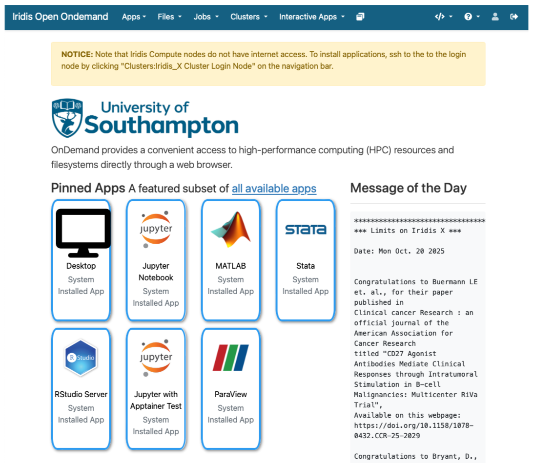
You can request access to Iridis on Demand through the same
application form to obtain an account on the system: here.
Simply include Iridis Ondemand keywords in the comment
section of the application.
Once granted access you can login at https://iridisondemand.soton.ac.uk/, ensuring you are on the campus network, or using the VPN.
Data Transfer
Moving data onto and from an HPC system can be achieved in several ways. One of the most common tools are SSH based SFTP (Secure File Transfer Protocol) and rsync.
Using SFTP in the terminal
Some extremely lightweight tools for data transfer exist, such as SFTP. It does however have some more advanced features than some of its lightweight rivals, including:
- Interactive sessions with remote file management such as renaming files, deleting files and directories and changing permissions and ownership.
- Providing better recovery mechanisms, such as being able to restart transfers from an interruption.
To start an interactive SFTP session on Iridis 6 from the terminal we can use the command:
Once connected you can:
-
list files:
sftp> ls -
change directories:
sftp> cd /path/to/remote/directory -
download a file:
sftp> get remote_file.txt /local/destination/ -
upload a file:
sftp> put local_file.txt /remote/destination/
SFTP can also be used non-interactively to transfer files:
rsync
rsync is another versatile command line based tool for
transferring data, it has a large number of options that allow for
flexible specification of the files to be transferred. It has a
delta-transfer algorithm, that compares modification times and sizes of
files to synchronise between storage locations by copying only files
that have changed and can allow restarting interrupted transfers.
For example to transfer a file from your system to Iridis 6:
where to option flags: - a archive option used to
preserve file timestamps and permissions - v verbose option
to monitor the transfer - z compression option to compress
the file during transfer - p partial option to preserve
partially transferred files in case of interruption
To recursively copy a directory you could use the following command:
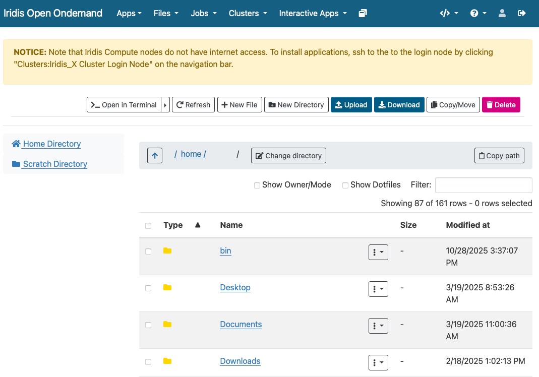
GUI based data transfer
There are GUI based alternatives to the above command line tools. One such option is Filezilla, a cross-platform client for MacOS, Windows and Linux that can use the SFTP protocol and will allow you to drag and drop files between the remote and local system.
Finally for Iridis X (and Iridis 6 as the two systems share a filesystem) Iridis on Demand has a file manager that will allow you to browse files as well as upload and download files to and from the system.
Data Management
Computational research can produce large quantities of complex data, and good data management is extremely important for the integrity and reproducibility of your research. Having a good handle on data management when using an HPC system will make your life as a researcher easier; it will help you avoid data loss, will reduce storage waste and make it easier to for you to locate and analyse your data.
Here are some suggestions for how to manage your data on an HPC system:
Organise your Data:
- Use clear directory structures, for example you could group by project, experiment, or date.
- Name files consistently: choose meaningful names that will help you identify what is in the file
- Use versioning tools such as git for code, scripts, configuration files and data.
- Include documentation such as README files and metadata alongside your data.
Use the right filesystem:
- Most HPC clusters provide multiple storage filesystems optimised for different purposes.
- Typically there will be a
homedirectory, which will be backed up. This space is best used for storing important source code, scripts, and essential datasets needed to run your jobs. - There will also likely be a
scratchspace on the file system. This area is designed for temporary or intermediate files — such as large simulation outputs or data requiring further analysis — that can be safely deleted or moved off the system once processing is complete. - Each system will differ, so check the documentation carefully
Data Lifecycle:
- Clean up old data to free up space: deleting or archiving with zipping tools.
- Track data provenance: Record how data was generated or modified.
- Back-up data: ensure important data is regularly backed up off the HPC system.
Iridis Filesystem & Quotas
Iridis 6 & X share a filesystem. On it you have access to two
main areas: - Home directory: (/home/username/):
backed up for important files - Scratch directory
(/scratch/username/): not backed up, for
temporary or intermediate input & output files to enable
computational workloads
There are two quota types in place on the system: - A data limit:
restricts the amount of data you can store. - 110 GB on
the /home/username/ directory - 1.5 TB on
the /scratch/username/ directory - An inode limit:
restricts the number of files you can store. - 160,000
on the /home/username/ directory -
*500,000 on the /scratch/username/
You can check the usage of the quotas with the following command on the system:
BASH
username@login6001:~$ myfiles
Home space used (GB): 24/130
━━━━━╸━━━━━━━━━━━━━━━━━━━━━━━━
Home number of files used: 202813/204800
━━━━━━━━━━━━━━━━━━━━━━━━━━━━━╸
Scratch space used (GB): 208/2000
━━━╺━━━━━━━━━━━━━━━━━━━━━━━━━━
Scratch number of files used: 486966/614400
━━━━━━━━━━━━━━━━━━━━━━━╸━━━━━━
If creating virtual environments (using e.g. conda or
python -m venv) it can be extremely easy to hit the inode
quota, so it is wirth remembering this command and regularly checking
your usage.
Software Management: Environment Modules
HPC systems will have a selection of centrally installed and managed software packages, but they will not be available to use immediately when you login. Software is usually managed on HPC systems using Environment Modules, and packages need to be loaded before they are available for use.
Challenge
There are several reasons behind the use of environment modules for software management. Can you think of any? Discuss it with your colleagues.
The three main reasons behind this approach:
- Software incompatibilities: Software incompatibility is a major headache for programmers. Sometimes the presence (or absence) of a software package will break others that depend on it. Two well known examples are Python and C compiler versions. Python 3 famously provides a python command that conflicts with that provided by Python 2.
- Versioning: Software versioning is another common issue. A team might depend on a certain package version for their research project - if the software version was to change (for instance, if a package was updated), it might affect their results. Having access to multiple software versions allows a set of researchers to prevent software versioning issues from affecting their results.
- Dependencies: Dependencies are where a particular software package (or even a particular version) depends on having access to another software package (or even a particular version of another software package).
Environment modules are the solution to these problems. A module is a self-contained description of a software package – it contains the settings required to run a software package and, usually, encodes required dependencies on other software packages.
There are a number of different environment module implementations commonly used on HPC systems: the two most common are TCL modules and Lmod. Both of these use similar syntax and the concepts are the same so learning to use one will allow you to use whichever is installed on the system you are using. In both implementations the module command is used to interact with environment modules. An additional subcommand is usually added to the command to specify what you want to do. For a list of subcommands you can use module -h or module help. As for all commands, you can access the full help on the man pages with man module.
On login you may start out with a default set of modules loaded or you may start out with an empty environment; this depends on the setup of the system you are using.
Listing Available Modules
In order to see what software modules are available we can use:
BASH
[username@login6002 ~]$ module avail
-------------------------------------------------------- /iridisfs/i6software/modules/applications --------------------------------------------------------
   GATK/4.1.9                      ansys/mechanical.2024.1        ensembl-vep/113              interproscan/5.71         paraview/5.10.1
   GATK/4.4.0                      ansys/mechanical.2024.2        fastq-tools/0.8.3            jdftx/1.7.0_gcc           paraview/5.12.1
   GATK/4.5.0                      ansys/mechanical.2025.1        fastqc/0.12.1                jdftx/1.7.0_mkl           paraview/5.13.3   (D)
   GATK/4.6.0                      ansys/mechanical.2025.2        ffmpeg/7.0.2                 jdftx/1.7.0        (D)    perl/5.40.0
   GATK/4.6.1                      ansys/polyflow.2024.2          gnuplot/6.0.1                julia/1.10.4              picard/3.3.0
   GATK/4.6.2               (D)    ansys/workbench.2024.2         gromacs/2022.5_plumed        julia/1.11.4              plink/1.9
   R/4.4.0-gcc8                    ansys/workbench.2025.1         gromacs/2024.1.dev1          julia/1.11.6              pycharm/2023.3.4
   R/4.4.1-mkl                     ansys/workbench.2025.2  (D)    gromacs/2024.1.amd           julia/1.11.7              python/3.12
   R/4.4.3-mkl                     bcl2fastq/2.20                 gromacs/2024.1.gcc           julia/1.12.1       (D)    python/3.12.6
   R/4.5.0-mkl                     bedtools/2.31.1                gromacs/2024.1.intel         lumerical/2024.2          python/3.13
   R/4.5.1-mkl              (D)    bionano/3.8.2                  gromacs/2024.1.zen4          lumerical/2025.1          python/3.14.0     (D)
   Rstudio/2024.09                 bison/3.8.2                    gromacs/2024.3.amd           lumerical/2025.2   (D)    samtools/1.20
   Rstudio/2024.12          (D)    blender/4.2.0                  gromacs/2024.3.intel         mathematica/14.0.0        silvaco/TCAD/2024
   Rstudio_server/2023.12.1        bwa-mem2/2.2.1                 gromacs/2024.5.amd           matlab/2024a              starccm/18.04
   Rstudio_server/2024.04.2 (D)    bwa/0.7.18                     gromacs/2024.5.intel         matlab/2024b       (D)    starccm/19.02
   STAR/2.7.11                     castep/25.1.2                  gromacs/2025.1.intel         namd/3.0.1                starccm/19.04
   abaqus/2024                     cfx/2025.1                     gromacs/2025.2.intel  (D)    nano/8.1                  starccm/19.06
   actran/2024.2                   comsol/6.1                     gurobi/11.0.3                nwchem/7.2.2_aocc         starccm/20.04     (D)
   ansys/fluent.2024.1             comsol/6.2_rev3                htslib/1.21                  nwchem/7.2.2_intel        stata/18.0
   ansys/fluent.2024.2             comsol/6.2                     hyperworks/2022.3            nwchem/7.2.2_ompi5        stata/19.0        (D)
   ansys/fluent.2025.1             comsol/6.3              (D)    hyperworks/2024.1            nwchem/7.2.2       (D)    tecplot/2023r1
   ansys/fluent.2025.2             csd/2024.1                     hyperworks/2025       (D)    onetep/7.2.intel          x13as/1.1
   ansys/forte.2024.1              datamash/1.3                   igv/2.19.1                   orca/6.1

--------------------------------------------------------- /iridisfs/i6software/modules/compilers ----------------------------------------------------------
   aocc/4.2             gcc/13.2.0    gcc/15.1.0        go/1.24.0                               intel-compilers/2024.1.0        nasm/2.16.03
   aocc/5.0      (D)    gcc/14.1.0    gcc/15.2.0 (D)    go/1.25.1                        (D)    intel-compilers/2025.0.0
   binutils/2.42        gcc/14.2.0    go/1.22.3         intel-compilers/2022.2.0.classic        intel-compilers/2025.1.0 (D)

----------------------------------------------------------- /iridisfs/i6software/modules/tools ------------------------------------------------------------
   apptainer/1.3.1    apptainer/1.4.2 (D)    cmake/3.30.5    cmake/4.1.1         (D)    gmsh/4.13.1        swig/4.3.0
   apptainer/1.3.6    awscli/v2              cmake/3.31.1    conda/python3              gocryptfs/2.5.4    valgrind/3.23.0
   apptainer/1.4.0    cmake/3.29.3           cmake/4.0.0     gdb-oneapi/2025.0.0        hpl/2.3

--------------------------------------------------------- /iridisfs/i6software/modules/libraries ----------------------------------------------------------
   aocl/4.2.0                  geos/3.13.0                     jdk/23.0.1                  openmpi/4.1.8                   sqlite3/3.46.1
   aocl/5.0.0                  gsl/2.8                         jdk/24                      openmpi/5.0.3_aocc              szip/2.1.1
   aocl/5.1.0_gcc14     (D)    guile/3.0.10                    jdk/25               (D)    openmpi/5.0.3_gcc13             tbb/2021.7.0
   boost/1.86.0                hdf5/1.14.5.classicintel        libfabric/1.22.0            openmpi/5.0.3_gcc14             tbb/2021.12
--More--
Loading a Module
Say we have written a C program, that uses the MPI (Message Passing
Interface) for parallel communication. Now we want to cmopile it with
the mpicc compiler. We can see if the path to the
mpicc compiler can be found in our shell with the
which command (which shows the full path of shell
commands):
BASH
[username@login6002 ~]$ which mpicc
/usr/bin/which: no mpicc in (/home/co1f23/.local/bin:/home/co1f23/bin:/opt/clmgr/sbin:/opt/clmgr/bin:/opt/sgi/sbin:/opt/sgi/bin:/usr/lpp/mmfs/bin:/usr/local/bin:/usr/bin:/usr/local/sbin:/usr/sbin:/iridisfs/i6software/slurm/default/bin:/iridisfs/i6software/slurm/bin:/opt/c3/bin)### What is $PATH? - $PATH is an
environment variable that tells your shell where to look for executable
programs when you type a command. It’s a list of directory paths,
separated by colons (:). When you run a command like mpicc, the system
searches these directories in order until it finds a matching
executable. - Loading modules (like openmpi) adds new directories to
$PATH, allowing you to use the software they provide
without typing the full path to the executable. - The system looks
through directories listed in our $PATH environment
variable for the shell commands. The directories are listed following
the no mpicc in message returned from the failed
which command above.
In order to load openmpi, a module containing
mpicc, we issue the following command:
Now when we use which to try and find the path to
mpicc we get a different result:
mpicc is now found, and if we look at our
$PATH environment variable we can see why:
BASH
[username@login6002 ~]$ echo $PATH
/iridisfs/i6software/openmpi/5.0.6/aocc_5/bin:/iridisfs/i6software/gcc/14.2.0/install/bin:/iridisfs/i6software/binutils/2.42/install/bin:/iridisfs/i6software/aocc/5.0/install/aocc-compiler-5.0.0/bin:/iridisfs/i6software/conda/miniconda-py3/condabin:/home/co1f23/.local/bin:/home/co1f23/bin:/opt/clmgr/sbin:/opt/clmgr/bin:/opt/sgi/sbin:/opt/sgi/bin:/usr/lpp/mmfs/bin:/usr/local/bin:/usr/bin:/usr/local/sbin:/usr/sbin:/iridisfs/i6software/slurm/default/bin:/iridisfs/i6software/slurm/bin:/opt/c3/bin
Several additions have been made to the list of directory paths the
sytem will search to find the commands we issue, including the one that
contains the mpicc command.
So, issuing the module load command will add software to
your $PATH. It “loads” software.
If we now look at the modules loaded we can see that the dependencies of the openmpi module have also been loaded:
Unloading Modules
In order to now unload the openmpi module we can use the command:
Now if we list the currently loaded modules:
we see that the openmpi module, along with its dependencies, have all been unloaded.
Getting Help
There are multiple avenues to getting help with Iridis.
You can find out more details about the system from the HPC Community Wiki.
There is a team of HPC system adminstrators that look after Iridis, including supporting the installation and maintenence of the software you need. You can contact them through the HPC Community Teams.
Research Software Group & HPC Research Software Engineers
The Research Software Group at Southampton is a team of Research Software Engineers (RSE) dedictaed to ensruing software developed for research is as good as it can be. We offer a full range of Software Development Services, covering many different technologies and all academic disciplines.
Within the Research Software Group there is a team of HPC RSEs who have been employed to help researchers make the best use of Iridis. Optimising or extending existing codes to make best use of the HPC resources available, e.g. refactoring, porting to HPC, porting to GPU.
You can get in touch with the group by emailing rsg-info@soton.ac.uk.
Access Iridis 6 and Iridis X requires applying for an account via a short online form, including project details and computing needs.
Iridis On Demand provides a web-based interface for accessing the HPC system, managing files, submitting jobs, and running interactive applications like Jupyter notebooks.
Connections to HPC systems are made securely using SSH (Secure Shell), typically through a public-private key pair for secure authentication.
Data transfer to and from HPC systems can be done using SSH-based tools such as sftp, or rsync, or through GUI tools like FileZilla or the Iridis On Demand.
Software on HPC systems is managed using Environment Modules, which allow users to load, unload, and switch between software packages and versions.
Help and documentation are available through the HPC Community Wiki, Teams HPC Community.
There is a team of Research Software Engineers in the Research Software Group whose role is to help researchers port and optimise code for use on HPC systems.
Content from Introduction to Job Scheduling
Last updated on 2025-11-04 | Edit this page
Estimated time: 0 minutes
Overview
Questions
- What is a job scheduler and why is it needed?
- What is the difference between a login node and a compute node?
- How can I see the available resources and queues?
- What is a job submission script?
- How do I submit, monitor, and cancel a job?
- How (and when) should I use an interactive job?
Objectives
- Describe briefly what a job scheduler does
- Contrast when to run programs on an HPC login node vs running them on a compute node
- Summarise how to query the available resources on an HPC system
- Describe a minimal job submission script and parameters that need to be specified
- Summarise how to submit a batch job and monitor it until completion
- Summarise the process for requesting and using an interactive job
An HPC cluster has thousands of nodes shared by many users. A job scheduler is the software that manages this, deciding who gets what resources and when. It ensures that tasks run efficiently and fairly, matching a job’s resource request to available hardware. On Iridis, the scheduler is Slurm, but the concepts are transferable to other schedulers such as PBS.

The scheduler acts like a manager at a popular restaurant. You must queue to get in, and you must wait for a table to become free. This is why your jobs may sit in a queue before they start, unlike on your computer. In this episode, we’ll look at what a job scheduler is and how you interact with it to get your jobs running on Iridis.
Can I run jobs on the login nodes?
On Iridis, and all HPC clusters, the login nodes are intended only for light and short tasks such as editing files, managing data, compiling code and submitting/monitoring jobs in the queue.
You must not run computationally intensive or long-running tasks on them. Login nodes are a shared resource for all users to access the system, and so running intensive jobs on them slows the system down for everyone. Any such process will be ended automatically, and repeated misuse may lead to your access to Iridis being restricted. To enforce this, login nodes have strict resource limits. You are limited to 64 GB of RAM and 2 CPUs (Iridis X also provides an NVIDIA L4 GPU).
All computationally intensive work must be submitted to the job scheduler. This places your job in a queue, and Slurm will allocate dedicated compute node resources to it when they become available. If you are compiling a large, complex codebase which requires more resources, or need to transfer large amounts of data, you should probably perform the tasks on a compute node instead. You can do this by submitting a job or by starting an interactive session, both of which we will cover later.
Querying available resources
Compute nodes in Slurm are grouped together and organised into
different partitions. You can think of a partition as
the actual queue for a certain set of hardware. Clusters are made up of
different types of compute nodes, e.g. some with lots of memory, some
with GPUs, some with restricted access, and some that are just
“standard” compute nodes. The partitions are how Slurm organises this
hardware. Each partition has its own rules, such as a maximum run time,
who can access the resources in it or a limit on the number of nodes
that can used at once. To find what the partitions are on Iridis 6 and
their current state, we can use the sinfo command:
BASH
[iridis6]$ sinfo -s
PARTITION             AVAIL  TIMELIMIT   NODES(A/I/O/T) NODELIST
batch*                   up 2-12:00:00      99/35/0/134 red[6001-6134]
highmem                  up 2-12:00:00          3/1/0/4 gold[6001-6004]
worldpop                 up 2-12:00:00          0/6/0/6 red[6135-6140]
scavenger                up   12:00:00          0/6/0/6 red[6135-6140]
interactive_practical    up   12:00:00          1/0/0/1 red6128
The -s flag outputs a summarised version of this list.
Omitting this flag provides a full listing of nodes in each queue and
their current state, which gets quite messy.
We can see the availability of each partition/queue, as well as the
maximum time limit for jobs (in days-hours:minutes:seconds
format). For example, on the batch queue there is a two and a half day
limit, whilst the scavenger queue has a twelve hour limit. The *
appended to the batch partition name indicates it is the preferred
default queue. The NODES column indicates the number of nodes in a given
state,
| Label | State | Description |
|---|---|---|
| A | Active | These nodes are busy running jobs. |
| I | Idle | These nodes are not running jobs. |
| O | Other | These nodes are down, or otherwise unavailable. |
| T | Total | The total number of nodes in the partition. |
Finally, the NODELIST column is a summary of the nodes belonging to a
particular queue; if we didn’t use the -s option, we could
get a complete list of each node in each state. In this particular
instance, we can see that 35 nodes are idle in the batch partition, so
if that queue fits our needs we may decide to submit to that as there
are available resources.
We can find out more details about specific partitions by using the
scontrol show command, which lets us view more
configuration details of a particular partition. To see the breakdown of
the batch partition, we use:
BASH
[iridis6]$ scontrol show partition=batch
PartitionName=batch
   AllowGroups=ALL DenyAccounts=worldpop AllowQos=ALL
...
   MaxTime=2-12:00:00 MinNodes=0
...
   State=UP TotalCPUs=25728 TotalNodes=134
...
   DefMemPerCPU=3350 MaxMemPerNode=650000
This purposefully truncated output shows who does and doesn’t have access (AllowGroups, DenyAccounts) as well as details about the configuration and details of the nodes in the partition (e.g. MaxTime, MinNodes, TotalNodes, TotalCPUs). Here, we can see accounts belonging to the “worldpop” group do not have access to the batch partition.
To get more detail about a particular node in a partition we use:
BASH
[iridis6]$ scontrol show node=red6001
NodeName=red6001 Arch=x86_64 CoresPerSocket=96
   CPUAlloc=192 CPUEfctv=192 CPUTot=192
...
   RealMemory=770000 AllocMem=643200 FreeMem=531885 Sockets=2
   State=ALLOCATED
...
   Partitions=batch
This provides a detailed summary of the node, including the number of CPUs on it (CPUTot), if there are GPUs (Gres) as well as the state of the node (State), the current resources allocated to a user (CPUAlloc, AllocMem) and other interesting information.
The scavenger partition
The scavenger partition on Iridis allows you to use idle compute nodes that you do not normally have access to, ensuring those resources do not go to waste. However, this access is low-priority. If a user with access to those nodes submits a job, your scavenger job will be preempted. This means your job is automatically cancelled and put back into the queue. The scheduler will try to run it again later when other idle resources become available.
Because your job can be cancelled at any time, you should only use this partition for testing or for code that can save its progress (a technique known as checkpointing). This way, you won’t lose work if your job is preempted.
Job submission scripts
To submit a job to run, we have to write a submission
script which contains the commands that we want to run on a
compute node. This is almost always a bash script, containing special
#SBATCH directives that tells Slurm what resources you need
to run your job. A very minimal example looks something like this:
BASH
#!/bin/bash

#SBATCH --partition=batch
#SBATCH --time=00:01:00
#SBATCH --nodes=1
#SBATCH --cpus-per-task=2

# This is the command that will run
pwd
Let’s break down this Bash script. The first line we need to include
is the #!/bin/bash shebang, which let’s Slurm know the
script is a Bash script. The next four lines starting with
#SBATCH are instructions to Slurm which tell it the
resources we’ve requested to run the job. In this case, we have included
the minimum batch directives you should include to submit a
job: the partition to run on, how long the job needs to run, the number
of nodes we require and the number of CPUs. The table below shows a list
of the most commonly used directives.
| Parameter | Description | Example Value |
|---|---|---|
--job-name |
Sets a name for your job. | --job-name=my_analysis |
--nodes |
Requests a specific number of compute nodes. | --nodes=1 |
--ntasks |
Requests a total number of tasks (e.g., MPI processes). | --ntasks=16 |
--ntasks-per-node |
Specifies the number of tasks to run on each node. | -ntasks-per-node=8 |
--cpus-per-task |
Requests a number of CPU cores for each task (e.g., for OpenMP threads). | --cpus-per-task=4 |
--time |
Sets the maximum wall-clock time for the job (HH:MM:SS). | --time=01:30:00 |
--partition |
Specifies the queue (partition) to submit the job to. | --partition=highmem |
--gres |
Requests generic resources, most commonly GPUs. | --gres=gpu:1 |
--output |
Specifies the file to write the standard output (STDOUT) to. | --output=job_output.log |
--error |
Specifies the file to write the standard error (STDERR) to. | --error=job_error.log |
--mail-user |
Your email address for job status notifications. | --mail-user=a.user@soton.ac.uk |
--mail-type |
Specifies which events trigger an email (e.g., BEGIN, END, FAIL, ALL). | --mail-type=END,FAIL |
More directives can be found in the Slurm documentation.
So why do we request ntasks or
cpus-per-task? We can think of a task in Slurm as being an
instance of a program. Some programs are designed to run one instance of
themselves, but use many CPU cores. For programs like this, we should
request one task and 16 CPUs.
Other programs are designed to run multiple independent instances that work in parallel. For programs like this, we’d request 16 tasks and with one CPU per task.
Finally, some programs have multiple instances each using many CPU cores.
The submission script contains everything the compute node needs to
run your program correctly, from start to finish. After the
#SBATCH parameters, which have to go before your
commands, you write all of the shell commands needed to prepare
the environment and launch your code, as if you were running it for the
very first time. We need to do this because jobs essentially run from a
blank slate. The environment is not configured, so we have to configure
it. This includes, but is obviously not limited to, setting environment
variables, loading software modules, activating virtual environments (if
required) and navigating to the correct directory.
A more complete submission script, for running a Python script, would look something like this:
BASH
#!/bin/bash

#SBATCH --job-name=python-example
#SBATCH --partition=batch
#SBATCH --time=04:00:00
#SBATCH --nodes=1
#SBATCH --ntasks=1
#SBATCH --cpus-per-task=1

# Optional: print useful job info
echo "Running on host: $(hostname)"
echo "Job started at: $(date)"
echo "SLURM job ID: $SLURM_JOB_ID"
echo "Number of CPUs: $SLURM_CPUS_PER_TASK"

# Load required modules
module purge
module load python/3.11

# Activate Python virtual environment
source ~/myenv/bin/activate

# Set any environment variables or configuration options
export PYTHONUNBUFFERED=1

# Move to job directory
cd $SLURM_SUBMIT_DIR

# Run the Python script
python my_script.py --input data/input.txt --output results/output.txt
In this example, python_job.sh, we
used the following script: my_script.py. In the submission script,
you will notice that we have used environment variables starting with
$SLURM_. These are set by Slurm when a job starts running
on a compute node. A complete list of them have be found in the Slurm
documentation.
No internet access on compute nodes
On Iridis, the compute nodes do not have access to the internet. If your job script tries to download files or access any online resource, it will hang and eventually fail. You should run any short tasks that require internet access (like downloading datasets) on the login nodes before you submit your job, or in an Iridis on Demand interactive session.
Submitting, monitoring and cancelling jobs
Submitting jobs
Once we have written our submission script, we submit it to the job
queue using the sbatch command, giving it the argument the
name of our submission script.
If all goes well, you should see some output which says “Submitted batch job” followed by a job ID, which a unique ID given to the job. We’ll use this ID to manage our job such as checking the status of it or cancelling it.
Test your script before submitting it
It is always good practice to test your submission script before submitting a large or long-running job. There is nothing more frustrating than waiting hours for your job to start, only to have it crash instantly because of a simple typo or error in the script.
A good way to do this is to submit a test job that requests minimal
resources, for example: --nodes=1,
--cpus-per-task=1 and --time=00:05:00. These
small, short jobs usually have a much shorter queue time. The goal is
not to test your code at scale or get results; it is only to confirm
that the script successfully loads its modules, finds its files, and
launches the program without immediately failing. Another option would
be to use the scavenger partition, which tends to have shorter queue
times.
Monitoring jobs
We can check on the status of jobs we’ve submitted by using the
squeue command. This will show us any jobs we have waiting
in the queue or are currently running. Let’s take a look in more detail.
To take a look at only our jobs, we use:
BASH
[iridis6]$ squeue -u $USER
JOBID   PARTITION  NAME      USER     ST  TIME  NODES  NODELIST(REASON)
715860  batch      example   ejp1v21  R   0:00  1      red6085
715558  batch      video_so  ejp1v21  PD  0:00  1      (Dependency)
By using -u $USER, where $USER is the
environment variable containing our username, we only see our jobs. If
we used just squeue, we would see all the jobs which are
either currently in the queue or are running for all users and
partitions. We can also use -j to query specific job IDs.
However we choose to use squeue, it prints the details of
jobs including the partition, user and also the state of the job (in the
ST column). In this example, we can see two jobs. One is in R, or
RUNNING, state and another is in PD, or PENDING, state. A job will
typically go through the following states,
| Label | State | Description |
|---|---|---|
| PD | PENDING | The jobs might need to wait in a queue first before they can be allocated to a node to run. |
| R | RUNNING | The job is currently running. |
| CG | COMPLETING | The job is in the process of completing. |
| CD | COMPLETED | The job has completed. |
For pending jobs, you will usually see a reason for why the job is
pending in the NODELIST(REASON) column. This can be for a variety of
reasons, such as the nodes requested for job not being available, that
there are jobs in front of it in the queue, or that the job depends on
another completing first. Once the job is running, the nodes that it is
running on will be displayed in this column instead. While the
squeue table lists the common states for a successful job,
jobs can also end in failure. You may see other states, such as F
(Failed) if your program terminated with an error, OOM (Out of Memory)
if it exceeded its memory request, or CA (Cancelled) if you or an
administrator stopped it.
If we want more detail about a job, we can use
scontrol show again:
BASH
[iridis6]$ scontrol show jobid=715860
JobId=715860 JobName=example.sh
   UserId=ejp1v21(32917) GroupId=fp(245) MCS_label=N/A
   ...
   JobState=RUNNING Reason=None Dependency=(null)
   ...
   RunTime=00:00:09 TimeLimit=00:01:00 TimeMin=N/A
   SubmitTime=2025-10-29T14:58:31 EligibleTime=2025-10-29T14:58:31
   StartTime=2025-10-29T14:58:32 EndTime=2025-10-29T14:59:32 Deadline=N/A
   Partition=batch AllocNode:Sid=login6002:1385285
   NodeList=red6086
   ...
   AllocTRES=cpu=1,mem=3350M,node=1,billing=1
   ...
   Command=/iridisfs/home/ejp1v21/example.sh
   StdErr=/iridisfs/home/ejp1v21/slurm-715860.out
   StdOut=/iridisfs/home/ejp1v21/slurm-715860.out
This detailed output confirms the JobState is RUNNING (though it could be PENDING if still in the queue or COMPLETED if it had already finished). With this output we can see exactly how long the job has been running (RunTime) against its maximum allowed time (TimeLimit). It also provides a complete history, showing when the job was submitted (SubmitTime), when it reached the front of the queue (EligibleTime), and when it started running (StartTime).
The scontrol output also shows precisely where the job
is running and what resources it has (Partition, NodeList, AllocTRES).
It also tells us what script is being run (Command) and where the output
for the job will be stored (StdErr, Stdout).
Cancelling jobs
Sometimes we’ll make a mistake and need to cancel a job. This can be
done with the scancel command, giving it the ID of the job
you want to cancel:
A clean return of the command indicates that the request to cancel
the job was successful. It might take a minute for the job to disappear
from the queue, as Slurm cleans it up. If we need to do something a bit
more dramatic and cancel all of our jobs, both running and pending then
we can use the -u flag to specify the user jobs we want to
cancel,
We can also refine this to cancel only pending jobs, whilst letting
running ones finish by using the -t state flag.
Submit, monitor and cancel a Python example
Now try all of this yourself with the Python example from earlier in the episode. You should use the the Python script my_script.py and the submission script python_job.sh.
Submit your job, check in on its status in the queue and then cancel it. The job should run for around five minutes, giving you enough time to do these three steps.
First, submit the python_job.sh script using the
sbatch command.
Make a note of the Job ID (e.g., 715861) that is returned. Check the
status of your job using squeue -u $USER. You should see
your job listed, likely in the PD (Pending) state.
BASH
[iridis6]$ squeue -u $USER
JOBID   PARTITION  NAME      USER     ST  TIME  NODES  NODELIST(REASON)
715861  batch      python_job  ejp1v21  PD  0:00  1      (Priority)
Finally, cancel the job using scancel and the Job ID you
noted.
Interactive jobs
We have so far been using Slurm to submit jobs to a queue and then
waiting for them to finish. However, on Iridis we can also start an
interactive jobs where we get direct access to compute nodes via a shell
session, letting us start the jobs directly from the command line. This
is incredibly useful for debugging code which isn’t working, or for
experimenting and testing, e.g. you may want to test your submission
script using bash ./job-script.sh.
To start an interactive session use the sinteractive
command. By default, this will give a single node for 2 hours, but this
can be changed with same job parameters in a job submission script,
e.g. sinteractive --time=05:00:00 --cpus-per-task=4,
This will start an interactive session on the L4 partition on Iridis
X, for 2 hours with 1 CPU. If sufficient resources are available, the
interactive job will start immediately, otherwise, it will need to queue
to start. As resources may not be available immediately to satisfy the
requirements of an interactive job, it is normally only practical to use
interactive jobs for short jobs of a few hours or less, running on a
couple of nodes. You may also want to use sinfo -s to query
which partitions have idle nodes, and use those.
Once the interactive session has started, you are logged into the node the job has been allocated and you can run commands from as if it were a terminal session on your own computer. You can even use GUI applications as long as X-forwarding has been setup correctly.
- The job scheduler (like Slurm) manages all user jobs to ensure fair and efficient use of the cluster.
- Login nodes are for light tasks (editing, compiling); compute nodes are for running scheduled, intensive jobs.
- Use
sinfoandscontrolto query the status of partitions (queues) and nodes. - A job script is a Bash script containing
#SBATCHdirectives (resource requests) and the commands to be run. - Use
sbatchto submit a job,squeueto monitor its status, andscancelto cancel it. - Use
sinteractiveto request a live terminal session on a compute node for debugging or interactive work.
Content from Introduction to Programmatic Parallelism
Last updated on 2025-10-22 | Edit this page
Estimated time: 0 minutes
Overview
Questions
- What is parallelisation and how does it improve performance?
- What are the different types of parallelisation?
- Why does synchronisation matter?
Objectives
- Describe the concept of parallelisation and its significance in improving performance
- Differentiate between parallelising programs via processes and threads
- Compare and contrast the operation and benefits of shared and distributed memory systems
- Define a race condition and how to avoid them
Parallel programming has been important to (scientific) computing for decades as a way to decrease how long a piece of code takes to run making more complex computations possible, such as in climate modelling, pharmaceutical development, aircraft design, AI and machine learning, and etc. Without parallelisation, these computations which would take years to finish can instead be completed in hours or days! In this episode, we will cover the foundational concepts of parallel programming. But, before we get into the nitty-gritty details of parallelisation frameworks and techniques, let’s first familiarise ourselves with the key ideas behind parallel programming.
What is parallelisation?
At some point you, or someone you know, has probably asked “how can I make my code faster?” The answer to this question will depend on the code, but there are a few approaches you might try:
- Optimise the code.
- Move the computationally demanding parts of the code from a slower, interpreted language, such as Python, to a faster, compiled language such as C, C++ or Fortran.
- Use a different theoretical/computational or approximate method which requires less computation.
All of these reduce the total amount of work the processor does. Parallelisation takes a different approach: splitting the workload across multiple processing units such as central processing units (CPUs) or graphics processing units (GPUs). Each processing unit works on a smaller batch of work simultaneously. Instead of reducing the amount of work to be done by, e.g. optimising our code, we instead have multiple processors working on the task at the same time.
Sequential vs. parallel computing
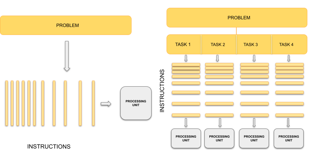
Traditionally, computers execute one instruction at a time, in the sequence defined by the code you have written. In other words, your code is compiled into a series of instructions which are executed one after another. We call this serial execution.
With parallel computing, multiple instructions, from the same program, are carried out at the same time on different processing units. This means more work is being done at once, so we get the results quicker than if we were running the same set of instructions sequentially on a single processor. The process of changing sequential code to parallel code is called parallelisation.
Painting a room
Parallel computing means dividing a job into tasks that can run at the same time. Imagine painting four walls in a room. The problem is painting the room. The tasks are painting each wall. The tasks are independent, you don’t need to finish one wall before starting another.
If there is only one painter, they must work on one wall at a time. With one painter, painting the walls is sequential, because they paint one wall at the time. But since each wall is independent, the painter can switch between painting them in any order. This is concurrent work, where they are making progress on multiple walls over time, but not simultaneously.
With two or more painters, walls can be painted at the same time. This is parallel work, because the painters are making painting the room by painting multiple walls at the same time.
In this analogy, the painters represent CPU cores. The number of cores limits how many tasks can run in parallel. Even if there are many tasks, only as many can progress simultaneously as there are cores. Managing many tasks with fewer cores is called concurrency.
Key parallelisation concepts
There is, unfortunately, more to parallelisation than simply dividing work across multiple processors. Whilst the idea of splitting tasks to achieve faster results is conceptually simple, the practical implementation is more complex. Adding additional CPU cores raises new issues:
- If there are two cores, they might share the same RAM (shared memory) or each have their own dedicated RAM (private memory). This distinction affects how data can be accessed and shared between processors.
- In a shared memory setup, what happens if two cores try to read or write the same memory location at the same time? This can cause a race condition, where the outcome depends on the timing of operations.
- How do we divide and distribute the workload evenly among the CPU cores? Dividing the workload unevenly will result in inefficient parallelisation.
- How will the cores exchange data and coordinate their actions? Additional mechanisms are required to enable this.
- After the tasks are complete, where should the final results be stored? Should they remain in the memory of one CPU core, be copied to a shared memory area, or written to disk? Additionally, which core handles producing the output?
To answer these questions, we need to understand what a process and what a thread is, how they are different, and how they interact with the computer’s resources (memory, file system, etc.).
Processes
A process is an individual running instance of a software program. Each process operates independently and possesses its own set of resources, such as memory space and open files, managed by the operating system. Because of this separation, data in one processes is typically isolated and cannot be directly accessed by another process.

One approach to achieve parallel execution is by running multiple coordinated processes at the same time. But what if one processes needs information from another processes? Since processes are isolated and have private memory spaces, information has to be explicitly communicated by the programmer between processes. This is the role of parallel programming frameworks and libraries such as MPI (Message Passing Interface). MPI provides a standardised library of functions that allow processes to exchange messages, coordinate tasks and collectively work on a problem together.
This style of parallelisation is the dominant form of parallelisation on HPC systems. By combining MPI with a cluster’s job scheduler, it is possible to launch and coordinate processes across many compute nodes. Instead of having access to just a single CPU or computer, our code can now use thousands or even tens of thousands of CPUs across many computers which are connected together.
Threads
A thread is a unit of execution which exists within a process. Unlike processes, threads share their parent process’ resources, including memory and open files, so they can directly read and write the same memory space. This shared access means threads can exchange data faster, since they do not have to communicate it between them.

By running multiple threads, over multiple CPU cores, a program can coordinate for each thread to work on their own task(s). For example, one thread may handle input/output whilst other threads perform some number crunching, or multiple threads might process different parts of a dataset simultaneously.
A major advantage of using threads is their relative ease of use compared to processes. With frameworks such as OpenMP), which provides a set of compiler extensions and libraries for paralleling code using threads, existing code can be adapted for parallel execution with, often, relatively small changes. Because threads share a memory space, there is no need for explicit message-passing mechanisms (as required with processes). However, this shared memory model introduces the possibility of race conditions, where two or more threads attempt to update the same data at once. Careful synchronisation is therefore required. It is important to note, however, that threads are confined to a single process and therefore to a single computer. Programs which are parallelised using threads cannot span across compute nodes in a cluster.
Shared vs distributed memory parallelisation
When writing parallel programs, a key distinction is whether there is a single shared memory space or if there are multiple private memory spaces. These two models are called shared memory and distributed memory.
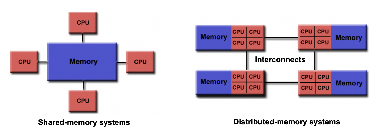
In a shared memory system, all processors (or cores) can directly access and modify the same pool of memory. Changes made by one processor are immediately visible to the others. This model aligns naturally with parallelisation using threads, which exist within a single process and share the parent process’ memory. However, shared memory has limitations: if multiple threads try to update the same data simultaneously, race conditions can occur. Correct results require careful synchronisation. Programming models such as OpenMP (Open Multi-Processing) provide mechanisms to divide work among threads and synchronise access to shared data. In general, shared memory approaches are generally limited to the cores within a single computer or node. The advantage of shared memory is its simplicity, making it easier to implement and debug. The main disadvantage is limited scalability, as performance gains are constrained by the number of cores in a single node and the complexity of synchronisation.
In a distributed memory system, each processor has its own private memory. Data cannot be accessed directly by other processors, it must be explicitly sent and received. This model aligns with parallelisation using processes which each have their own private memory space. Communication between processes is typically handled using libraries such as MPI. Distributed memory programming requires more effort than shared memory, but it enables programs to scale across multiple nodes in a cluster. The advantage of distributed memory is its high scalability, allowing computations across thousands of nodes. The disadvantages include increased programming complexity and additional overheads required for communication information, as data must be explicitly exchanged between processes (private memory spaces).
The differences can be summarised:
- Accessibility: Shared memory allows direct access to a common memory space. Distributed memory requires explicit communication for data exchange.
- Memory scope: Shared memory provides a global pool, while distributed memory isolates each processor’s memory.
- Consistency: In shared memory, changes are immediately visible to all cores. In distributed memory, explicit synchronisation is needed to keep results consistent.
- Scalability: Shared memory is limited to one node. Distributed memory scales to thousands of nodes.
- Programming complexity: Shared memory models are simpler to use but harder to scale. Distributed memory models scale well but require more explicit programming.
- Advantages/Disadvantages: Shared memory is easier to program , but is limited in scale and prone to synchronisation issues. Distributed memory scales to more cores, but is more complex and requires explicit data communication.
In sophisticated applications, a hybrid approach is used which combines using processes to spread the workload across multiple nodes, but uses shared-memory parallelisation on a node. This takes advantage of the scalability of distributed memory, and the efficiency of using shared-memory with threads.
Synchronisation and race conditions
Synchronisation ensures that processing units can coordinate their actions correctly, particularly when threads are accessing or modifying shared data. Without proper synchronisation, multiple threads, for example, might attempt to update the same variable simultaneously, leading to unpredictable results known as a race condition.
In a shared memory system, synchronisation mechanisms such as barriers, locks, and atomic operations are used to control access to shared data and to coordinate work. A barrier ensures that threads have reached a certain point before continuing, while locks prevent sections of code from being executed simultaneously, preventing race conditions. Atomic operations allow individual updates to shared variables without interference, meaning only one thread can update a variable at once. Proper use of these mechanisms ensures code correctness, maintaining consistent and valid results.
In distributed memory systems, synchronisation is achieved by coordinating communication between processes to order the workload and manage data dependencies. Even though processes have their own private memory space, race conditions can still occur if two processes write to the same file. Effective synchronisation, whether with threads or processes, is crucial for ensuring that parallel programs produce correct, reproducible results.
Organising the painters
Imagine several painters working on the same set of walls. If each painter tries to paint the same wall at the same time without coordinating, they might overwrite each other’s work creating a mess. This is like a race condition in parallel programming, where there is simultaneous memory access modifying the same data.
To avoid this, painters might take turns for the shared wall, or divide walls so each painter works independently. In programming, mechanisms like barriers or atomic operations perform the same role: they synchronise access to shared resources.
This coordination ensures that all parts of the task progress in the right order, whether you are updating a shared variable, writing results to disk, or aggregating data.
- Parallelisation speeds up computation by dividing work across multiple processing units.
- Processes use private memory and communicate information explicitly between them (distributed memory, e.g. MPI).
- Threads share memory within a process and require synchronisation to prevent race conditions.
- Shared memory parallelisation is simpler but limited in scale. Distributed memory scales better, but is more complex.
Content from Landscape of HPC Technologies
Last updated on 2025-11-06 | Edit this page
Estimated time: 0 minutes
Overview
Questions
- Which programming language should I use?
- What are the main ways we can parallelise a program on modern HPC systems?
- How do OpenMP and MPI differ in how they achieve parallelism?
- What role do GPUs play in HPC, and how do approaches like CUDA and OpenACC use them?
Objectives
- Differentiate at a high level between the features of OpenMP, MPI, CUDA and OpenACC
- Briefly summarise the main OpenMP compiler directives and what they do
- Describe how to compile and run an OpenMP program
- Briefly summarise the main MPI message-passing features and how they are used
- Describe how to compile and run an MPI program
- Briefly summarise how an OpenACC program is written, compiled and run
- Briefly summarise how a CUDA program is written, compiled and run
To get the most performance possible, high-performance computing relies on parallelism. Modern systems combines tens of thousands of processors, each working on their own part of the problem. To be able to wield this power, we need to understand how to write parallel code. This is far more complicated than the scope of this episode. Therefore we will, instead, look at the landscape of the core HPC technologies used today in research. In particular, we will look at the following parallel frameworks: OpenMP, MPI, OpenACC and CUDA.
Common programming languages
Before we start, let’s look at what programming languages are used in HPC. In principle, any programming language can be used to write code which runs on an HPC cluster. In practise, however, there are some languages which are better suited to writing highly performant code. Interpreted languages, such as Python, are easy to develop in, but are much slower to execute than compiled languages, making them less suitable for computation-heavy applications. For this reason, compiled languages such as C, C++ and Fortran are some of the most common choices of programming language when writing high performance applications as they produce fast, optimised executables.
Python does, however, remain widely used in HPC, typically by performance-critical sections of code being written in compiled languages and accessed through a Python interface. Frameworks such as PyTorch, NumPy, SciPy and Numba all rely on underlying C, Fortran and/or CUDA to accelerate computation, while libraries such as mpi4py or multiprocessing make it possible for distributed parallelism directly in Python. Hybrid approaches like this have become more common because they combine Python’s ease of use with the speed of compiled code.
Other specialised languages and frameworks are also used in HPC, depending on the application area. CUDA and ROCm are employed for GPU programming, while newer languages such as Julia aim to combine ease of development with high performance. Domain-specific tools like MATLAB, and R also appear in HPC environments, though they often rely on compiled extensions or external libraries for parallel execution.
So which language should you use? There is no simple answer. The best choice depends heavily on your specific application, the target hardware (like CPUs or GPUs), and the trade-offs you are willing to make between raw computational performance and ease of development. Ultimately, the right language is the one that allows you to solve your problem efficiently, leveraging the available libraries and expertise within your team.
Which compiler should you use?
Iridis and most HPC systems offer a choice of compilers to use. But
which one should you use? In most cases, you would want to use the
compiler specific to the type of CPU you are using on the system,
because these implement architecture specific optimisations e.g. use
AMD’s aocc on Iridis 6. If you are using NVIDIA GPUs, you
have little choice in using anything other than NVIDIA’s
nvc, nvcc or nvfortran
compilers.
However, the code you are using may only have been tested on a specific compiler such as GCC. In those cases, it’s often best to stick with what is known to work. However, there is nothing stopping you using Intel’s compilers on an AMD based system, if the code is only tested or depends on features in the Intel compilers.
A simple example
We’ll now take a high level look at a selection of some of the most used libraries and frameworks used to parallelise code in research. In particular, we will see how to use them, the code changes required and how to run them on Iridis. The intention is not to make you proficient with these frameworks–or even dangerous–but to give a high level appreciation on what is being used.
To illustrate this, we will use a simple program, written in C, which
adds together two vectors to explore the code changes required. More
specifically, we will be modifying the following function
vector_add to run in parallel. We have chosen to use C as
it is commonly used language in HPC.
C
// *a, *b, and *c are arrays and n is the length of them.
// The result of the addition is returned back in *c
void vector_add(int *a, int *b, int *c, int n) {
    // This is the loop which we'll parallelise
    for (int i = 0; i < n; ++i) {
        c[i] = a[i] + b[i];
    }
}
You can find the entire program in vector_serial.c. To run this code on Iridis X, we’ll use the following submission script.
BASH
#!/bin/bash

#SBATCH --partition=amd
#SBATCH --nodes=1
#SBATCH --ntasks=1
#SBATCH --time=00:01:00

# Load the gcc module, which is the compiler we'll use
module load gcc

# Compile the program using gcc
gcc vector_serial.c -o vector_serial.exe

# Run the compiled executable
./vector_serial.exe
After the program has run, we should see the following output.
OUTPUT
Verification (first 5 elements):
c[0] =   0 (expected:   0)
c[1] =   3 (expected:   3)
c[2] =   6 (expected:   6)
c[3] =   9 (expected:   9)
c[4] =  12 (expected:  12)
OpenMP
The first framework we’ll look at is OpenMP. As mentioned in the previous episode, OpenMP is an industry-standard framework designed for parallel programming in a shared-memory environment. OpenMP spawns threads with each one, ideally, running on its own CPU core. OpenMP works by using compiler directives to tell the compiler which code needs to be parallelised, letting OpenMP and the compiler take care of all the low-level parallelisation details. In general, you just need to say which parts of your code you want to run in parallel.
Compiler directives
If you’re unfamiliar with compiler directives, you can think of them
as being a special command for the compiler, not for the
program itself. In C and C++, these almost always start with
#pragma. Think of it as a special note to the compiler
which says, “when you compile this specific piece of code, do something
extra.” Since these are compiler options, they do not modify the run
time behaviour of the program, only how the program is compiled.
Parallelisation with OpenMP is handled with these compiler
directives. However, OpenMP does also offer a library of runtime
functions which gives finer grained control, such as if you need to
ensure thread synchronisation or need to go off the beaten track. To
parallelise our vector_add function, we only need to add a
single line of code, using a compiler directive, just before the
loop.
C
void vector_add(int *a, int *b, int *c, int n) {
// This directive tells OpenMP to spawn threads and to
// divide the loop iterations between them. Each thread will
// handle a fraction of the loop iterations/vector addition
#pragma omp parallel for
    for (int i = 0; i < n; ++i) {
        c[i] = a[i] + b[i];
    }
}
The full program is in vector_openmp.c. Let’s break
this down more. The directive we used,
#pragma omp parallel for, tells the compiler that the next
for loop should be parallelised. The compiler then automatically
parallelises it for us, creating a team of threads and dividing the
loop’s work among them. In this case, each thread will perform a portion
of the vector addition. All OpenMP directives begin with
#pragma omp, followed by a specific command.
There are lots of other directives available, with
#pragma omp parallel for being the most commonly used.
Another useful directive is #pragma omp atomic which
prevents multiple threads from modifying a variable at once. This is one
way to prevent the race conditions mentioned in the previous episode.
OpenMP also provides a library of runtime functions which offers even
more control. For example, we can use the function
omp_set_num_threads() to control the number of threads that
OpenMP will spawn. In C, we need to include the appropriate header file,
<omp.h>, to access the library functions.
C
#include <omp.h>

void vector_add(int *a, int *b, int *c, int n) {
    // Manually set the number of threads to 8
    omp_set_num_threads(8);

#pragma omp parallel for
    for (int i = 0; i < n; ++i) {
        c[i] = a[i] + b[i];
    }
}Directives and functions for synchronisation
Effective control of thread synchronisation is essential when parallelising code with OpenMP, as improper handling of shared data can lead to race conditions and unpredictable results. To support this, OpenMP provides a range of directives and library functions that coordinate access to shared data and manage thread behaviour. The tables below summarise several commonly used examples.
| Compiler Directive | Description |
|---|---|
#pragma omp atomic |
Ensures a specific operation, such as modifying a variable, is executed atomically, e.g. by one thread at a time, to prevent race conditions. |
#pragma omp critical |
Defines a region of code that only one thread can execute at a time. |
This list is not exhaustive. A complete reference for all OpenMP directives and functions is available in the OpenMP 6.0 Reference Guide.
To compile an OpenMP program, we need to use the
-fopenmp flag,
e.g. gcc -fopenmp vector_openmp.c. If we don’t use the
-fopenmp flag, the compiler directives are ignored and any
library functions from <omp.h> will not be found
resulting in a compilation error.
Do I need to keep the serial version?
Setting the number of threads or processes to one will produce the
same behaviour as the serial program, assuming no programming errors.
However, to be extra safe, you can use conditional
compilation to maintain both parallel and serial versions within the
same codebase/file. Compiled languages support conditional compilation,
which allows certain sections of code to be compiled only if a specific
condition is met. When using OpenMP, the compiler variable
_OPENMP is defined when the -fopenmp flag is
passed, so you can use this variable to prevent OpenMP directives and
functions from being compiled when -fopenmp is not
used.
To launch an OpenMP program, run it like any other program. The
number of threads for OpenMP to use can be controlled using the
environment variable OMP_NUM_THREADS, or the
omp_set_num_threads() function discussed earlier. If the
function is unused and the environment variable left unset, OpenMP will
spawn one thread per CPU core. Normally, on a HPC cluster this is
probably what is wanted. However, when running on your own computer
during development and testing, you will probably want to set
OMP_NUM_THREADS to be less than then number of CPU cores to
avoid overloading your computer.
The following is an example of how you would compile and launch an OpenMP program on Iridis X, in a single submission script.
BASH
#!/bin/bash

#SBATCH --partition=amd
#SBATCH --nodes=1
#SBATCH --ntasks=1
#SBATCH --cpus-per-task=8
#SBATCH --time=00:01:00

# Use OMP_NUM_THREADS to say we can to use --cpus-per-task number of
# threads. The --cpu-per-task SBATCH directive is populated into the
# SLURM_CPUS_PER_TASK environment variable
export OMP_NUM_THREADS=$SLURM_CPUS_PER_TASK

# Compile the program using gcc
module load gcc
gcc -fopenmp vector_openmp.c -o vector_openmp.exe

# We run the compiled executable just like the serial version
./vector_openmp.exe
The main advantage of OpenMP is that it requires only minimal code modification to parallelise existing programs, particularly when the main computational workload lies within loops. Beyond simple loop-level parallelism, parallelising more complex program structures becomes more challenging, though this is true of most parallel frameworks. OpenMP still provides a wide range of straightforward directives, making it easy to adapt serial code without needing to design the program for parallel execution from the start. Its main limitation is that it uses a shared-memory model, which requires careful management of thread synchronisation and restricts scalability to a single compute node.
Message Passing Interface (MPI)
The Message Passing Interface (MPI) was designed to enable scientific applications to run on supercomputers and, as such, has become the dominant distributed-memory parallelism framework in research. An MPI application creates many processes each working on their own individual task. However, unlike shared-memory approaches, each MPI process–or rank–has its own private memory space. Therefore to exchange data between these ranks, explicit communication has to happen. This is where MPI comes in. It provides a set of library functions to configure a parallel environment and exchange data within it. The key concept in MPI is message passing, which involves the explicit exchange of data between processes. Processes can send messages to specific destinations, broadcast messages to all processes, or perform collective operations where all processes participate.
To achieve parallelism, each process runs a copy of the same program as the other processes, but works on its own subset of data, or does its own tasks. The processes communicate to exchange data and/or coordinate their next tasks. The power of MPI is that the processes can run on different nodes, allowing MPI programs to scale well beyond a single machine. Thankfully the complexity of having to spawn processes on different nodes and communicate over the network is hidden away and controlled by MPI’s library of functions and the HPC cluster’s scheduler/resource manager, e.g. Slurm on Iridis.
But there are some trade-offs with MPI. In terms of performance, communicating data takes time. If you have a method which requires frequent communication or data dependencies, then you will spend more time exchanging data than doing computation. It may instead be worth using a shared-memory framework like OpenMP. However the biggest trade-off, by far, is that you need to design your application in mind for MPI parallelisation. Unlike OpenMP, it is not simple to retrofit a serial program with MPI. For example, we need to make sure we program initialising the MPI library ourselves, track process IDs, explicitly send and receive data, coordinate the processes so they do their own work, and so on. The table below gives an idea of some of the MPI functions we need to use and their purpose.
| Function | Description |
|---|---|
MPI_Init |
Initialises the MPI environment. Must be called before any other MPI calls. |
MPI_Comm_size |
Returns the total number of processes in the communicator. |
MPI_Comm_rank |
Returns the rank (ID) of the calling process. |
MPI_Send / MPI_Recv
|
Used for direct point-to-point communication between processes. |
MPI_Barrier |
Used for synchronisation. A processes cannot continue past the barrier until all processes have reached it. |
MPI_Finalize |
Shuts down the MPI environment. Must be called before exiting the program, other wise background MPI tasks may not finish. |
This is only a tiny glimpse into the available MPI functions, and what you can do with MPI. In total, there are around 500 functions.
Let’s now take a look at the code changes we need to parallelise the
add_vector function using MPI. A detailed description of
the MPI library functions, and how to design an MPI program, is out of
scope for this episode, and lesson, so we won’t go much into the
details. From a high level, what we need to do is: 1) initialise the MPI
environment, 2) split the work between processes, 3) have each process
do their work, and 4) communicate the results back to one or more
processes for the cycle to repeat. The example code below demonstrates
this. Keep in your head that each process is executes the
exact same function, but will do something different
based on its ID.
C
//Include the MPI header file to access the MPI functions
#include <mpi.h>

void vector_add(int *a, int *b, int *c, int n) {
    // Initialise the MPI environment -- nothing will work if we
    // don't do this
    MPI_Init(NULL, NULL);

    // Get the rank (process ID) and total number of processes launched
    int rank, size;
    int root_rank = 0;
    MPI_Comm_rank(MPI_COMM_WORLD, &rank);
    MPI_Comm_size(MPI_COMM_WORLD, &size);

    // Determine next how many elements of the vector this process
    // will handle. We will create a "local" array which will store
    // the results of the vector addition for this process
    int n_local = n / size;
    int c_local[n_local];

    // Determine the subset of the vectors a and b this process
    // will be adding together. To do this, we use the ID of
    // the process and the number of elements each process
    // will be working on
    int start = rank * n_local;
    int stop = (rank + 1) * n_local;

    // Perform the local computation on each process
    for (int i = start; i < stop; i++) {
        c_local[i] = a[i] + b[i];
    }

    // We can use this MPI_Gather function to send the "partial" results
    // from each process back to the "root" process. Only the root process
    // will have the complete vector
    MPI_Gather(c_local, n_local, MPI_INT, c, n_local, MPI_INT,
               root_rank, MPI_COMM_WORLD);

    // Finalise the MPI environment
    MPI_Finalize();
}
The complete program is in vector_mpi.c. As you can see, the code is much more involved than the OpenMP example. Every process runs this same function, but each one is responsible for a different part of the vector addition. Each process follows a clear set of steps:
- First, it finds out its unique ID (
rank) and the total number of processes (size). - Using this, it calculates which “slice” of the vectors
aandbit is responsible for. - It then performs the addition for its slice and stores the partial
answer in a local
c_localarray. - Finally, it calls the
MPI_Gatherfunction, which aggregates all thec_localarrays.
MPI_Gather is a collective communication shortcut.
Behind the curtain it doing the MPI_Send and
MPI_Recv for us, sending data from each process back to our
root process; which is the only process with the complete result.
Challenge
Why does only the “root” process have the final, complete, result?
It is because we used MPI_Gather to “gather” the results
from each process back to the root process. There is no communication to
the other process, so only the root process has the data from the other
processes. If we wanted every process to have a copy of the final result
of c, we could instead use MPI_Allgather.
To compile an MPI application, we need to use an MPI-aware
compiler which is essentially a clever script which knows where MPI is
installed on our system to make compilation easier. On Iridis, this is
mpicc. We use mpicc as we would any other
compiler: mpicc vector_mpi.c -o vector_mpi.exe.
What’s an MPI-aware compiler?
An MPI-aware compiler is essentially a script which wraps around your
regular compiler to provide the required header files and libraries to
the compiler to build an MPI application. In theory, we could find those
headers and libraries ourselves and pass them the compiler instead.
However, in practise, this is not worth our time when mpicc
already does it for us.
To launch an MPI application we need to use mpirun,
e.g. mpirun vector_mpi.exe. This is another script provided
by MPI which handles launching the parallel processes and setting up the
parallel environment. If we run the program without using
mpirun, then only a single processes will start and will
probably become “deadlocked” as the program waits indefinitely for
messages from other processes that were never sent. On Iridis, and other
Slurm clusters, we can alternatively use the Slurm launcher
srun to do the same job. To summarise, the purposes of
srun and mpirun is to,
- Read the environment to see how many processes to create (e.g., from
#SBATCH --ntasks=8). - Launch that many copies of your executable.
- Manage where these processes run. If you request resources across multiple nodes, the launcher (in coordination with Slurm) starts the processes on the correct machines and ensures they can all communicate with each other.
The following is an example of how you would compile and launch an MPI program on Iridis X.
BASH
#!/bin/bash

#SBATCH --partition=amd
#SBATCH --nodes=1
#SBATCH --ntasks=8
#SBATCH --cpus-per-task=1
#SBATCH --time=00:01:00

# Load the specific MPI library we want to use
# This makes the 'mpicc' and 'mpirun' commands available
module load openmpi

# Compile the code using the MPI compiler wrapper
mpicc vector_mpi.c -o vector_mpi.exe

# Launch the program using 'srun'. This is the recommended
# launcher on Slurm clusters. 'srun' automatically reads the
# SBATCH settings and launches 8 (from --ntasks) copies
# of our executable
srun ./vector_mpi.exe

# -----------------------------------------------------------
# An alternative way to launch the program
# 'mpirun' is the more traditional MPI launcher. Here, we
# must explicitly tell it how many processes (-np) to run
# We use the $SLURM_NTASKS variable (which Slurm sets to 8)
# to match our resource request
# mpirun -np $SLURM_NTASKS ./vector_mpi.exe
# -----------------------------------------------------------Hybrid MPI+OpenMP
MPI and OpenMP don’t have to be competing choices. They can be used together in a hybrid parallel model, where MPI distributes work across nodes and OpenMP manages threads within each node. This combination allows applications to scale beyond a single machine while using memory and CPU cores more efficiently.
Hybrid parallelism reduces data duplication between processes and improves load balancing through OpenMP’s flexible scheduling. It also helps lower communication costs by keeping shared-memory operations local to a node.
The main drawbacks are added complexity and potential overheads from managing both models. Code becomes harder to write, debug, and port between systems. Still, hybrid MPI+OpenMP programs are often the best solution for large-scale workloads where pure MPI or OpenMP alone falls short.
Challenge
Why does using a hybrid MPI+OpenMP scheme reduce data duplication?
In a pure MPI application, you would run many separate processes on a single compute node (e.g., 64 processes on 64 cores). Each MPI process has its own private memory. If all 64 processes need to access the same 10GB input file, that 10GB of data must be loaded 64 times, once into each process’s memory. This duplicates the data 64 times, using 640GB of RAM on that node just for that one file.
In a hybrid MPI+OpenMP model, you may run only one MPI process on that node. That single process would then use OpenMP to spawn 64 threads, one for each core. Because all OpenMP threads share the memory of their parent process, the 10GB input file only needs to be loaded once. All 64 threads can access that single copy, reducing the memory footprint for that data from 640GB to just 10GB.
Using GPUs instead of CPUs
Besides using multiple CPUs, we can also use Graphical Processing Units (GPUs) to do calculations in parallel. GPUs were originally designed to speed up rendering to display images to a screen, a task that involves performing millions of simple, repetitive calculations in parallel. Researchers soon realised this design was also perfect for many scientific problems.
GPUs are highly parallel, built to perform thousands of operations at the same time. This makes them ideal for work that can be split into many identical, independent tasks. While CPUs are designed to tackle complex tasks one after another, GPUs are optimised for doing the exact same operation on large amounts of data simultaneously. This is perfect for problems like matrix operations, where every element can be processed in the same way.
However, offloading work to a GPU is more complicated than parallelising using CPUs. The main reason is that the CPU and the GPU have their own separate memory spaces. Data stored in the CPU’s memory is not visible to the GPU, and vice-versa. This setup is similar to the separate memory for each process in an MPI application. Data must be copied from the CPU’s memory to the GPU’s memory. This transfer step is slow compared to the speed of the calculations. Therefore, efficient GPU programs must minimise data transfers, often by keeping data on the GPU as long as possible. While optimising CPU code often focuses on reducing the total number of calculations, optimising GPU code is usually more about reducing data transfers and organising data efficiently in the GPU’s memory.
This level of detail is beyond the scope of this introduction. As before, we will only give a broad overview of two popular frameworks: OpenACC and CUDA. You can think of these as being similar to OpenMP and MPI:
- OpenACC is like OpenMP: you can often add it to existing code, using compiler directives to automatically handle the parallelisation.
- CUDA is “similar” to MPI: it is a more complex framework that requires you to design your program around it.
CPU and GPU, what’s the difference?
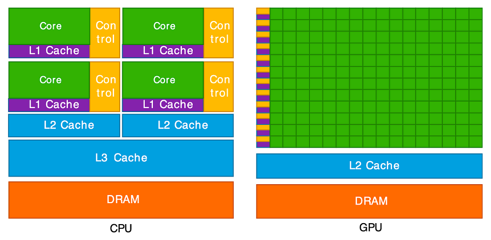
This diagram illustrates the key difference between a CPU and a GPU. On the left, the CPU is shown with a few, large “Cores” (green). Each core is complex, paired with significant “Control” logic (yellow) and large, fast memory caches (purple and blue). This design makes each CPU core very “smart” and powerful, ideal for handling complex instructions and varied tasks one after another.
On the right, the GPU has a completely different structure. It is
composed of hundreds or even thousands of tiny, simple cores (the large
green grid). Notice how much less space is dedicated to “Control” logic
and complex caches. This architecture is not designed for complex,
sequential tasks. Instead, it is a massive parallel workforce, built to
execute the same simple operation (like c[i] = a[i] + b[i])
at the same time across thousands of different pieces of data. This
“many-core” design is what allows it to perform thousands of operations
concurrently.
GPUs also use a different memory model. Each GPU core can access the large global memory, which is shared across the entire GPU. It is slower to read and write to this. To improve performance, groups of cores are organised into blocks which shared a small, but very fast, memory area. This setup is similar to shared-memory parallelism on CPUs, where threads cooperate through a common memory space. However, each GPU block’s shared memory is private to that block, much like how separate processes in a distributed-memory model (such as MPI) each have their own memory and must explicitly exchange data. Efficient GPU programs manage this hierarchy carefully, reusing shared memory to reduce costly access to global memory.
OpenACC
OpenACC is a framework for parallel programming on GPUs, both for NVIDIA and AMD GPUs; i.e. it is platform agnostic. Just like OpenMP, it uses compiler directives to tell the compiler which parts of code should be executed in parallel on a GPU. Also like OpenMP, the OpenACC runtime and compiler handles all of the parallelisation details such as generating the parallel code, transferring data between the CPU and GPU and synchronising/managing GPU threads.
Whilst most of the heavy lifting for OpenACC is done with compiler
directives, a runtime library is also available for finer control over
things such as selecting which GPU to use (if you are lucky enough to
have more than one!), finer grained data movement and synchronisation
mechanisms. To parallelise our vector_add function to a
GPU, we only need to add a single line of code.
C
void vector_add(int *a, int *b, int *c, int n) {
// This OpenACC directive tells the compiler to parallelise the
// following 'for' loop, running its iterations concurrently
// on the GPU
#pragma acc parallel loop
    for (int i = 0; i < n; ++i) {
        c[i] = a[i] + b[i];
    }
}
The full program is in vector_openacc.c. The directive
#pragma acc parallel loop tells the compiler to parallelise
the loop and execute it on the GPU. Each GPU core/thread performs part
of the vector addition. OpenACC also takes care of allocating memory on
the GPU and transferring data from the CPU to GPU’s memory. It also
copies the results back to the CPU when the loop is completed.
Some other useful directives
As we’ve seen,#pragma acc parallel loop targets a single
loop. OpenACC also provides the #pragma acc kernels
directive. This directive is meant to be put before a larger region of
code, such as a complicated loop or multiple loops. The compiler then
analyses this entire region and automatically determines the best way to
convert the code, including any loops it finds, into parallel “kernels”
of code to run on the GPU.
The main difference is that #pragma acc parallel loop is
prescriptive: you are explicitly telling the compiler to parallelise
that one loop. In contrast, #pragma acc kernels is
descriptive: you are telling the compiler “here is a block of code to
accelerate,” giving it freedom to analyse the code and choose the most
efficient way to parallelise and run it.
Additionally, whilst OpenACC automatically manages data transfers
between the GPU and CPU, more explicit data management is possible using
directives such as #pragma acc data, copy,
copyin, and copyout for more control.
To compile an OpenACC program, we need a compiler that supports it.
On Iridis X this is either GCC or one from NVIDIA’s compiler collection.
With GCC we need to use the -fopenacc flag. However, when
using NVIDIA’s C compiler, nvc, the flag is instead
-acc, e.g. nvc -acc vector_openacc.c. Without
the flag, the OpenACC directives are ignored and GPU code is not
generated.
The following is an example of how you would compile and launch an
OpenACC program on Iridis X. It is especially important that we remember
to request a GPU using the --gres=gpu:1 directive and
select a partition where nodes have GPUs.
BASH
#!/bin/bash

#SBATCH --partition=l4
#SBATCH --nodes=1
#SBATCH --ntasks=1
#SBATCH --cpus-per-task=1
#SBATCH --gres=gpu:1
#SBATCH --time=00:01:00

# Load the NVIDIA HPC SDK module, which provides OpenACC support
module load nvhpc

# Compile the program with GPU offloading enabled
nvc -acc vector_openacc.c -o vector_openacc.exe

# Check GPU availability and run the program
nvidia-smi
./vector_openacc.exe
The main advantage of OpenACC, like OpenMP, is that it allows rapid GPU parallelisation with minimal code changes. It is particularly useful for incrementally porting existing CPU applications to GPUs. However, compared to lower-level frameworks like CUDA, it offers less fine-grained control over GPU execution and memory management. OpenACC is therefore well suited for scientific and engineering applications where productivity are more important than maximal performance.
CUDA
The final framework we will look at is CUDA, which is essentially a programming language created by NVIDIA to run arbitrary code on NVIDIA GPUs. However, unlike OpenACC which uses compiler directives to automatically parallalise sections of code, CUDA is an extension of the C/C++ language which gives you explicit fine-grained control over the GPU. This is a much more powerful and performant approach, but also far more complex. You are no longer advising the compiler; you are directly writing the code that will run on the GPU. Given this complexity, we will only examine the key concepts at a very high level.
In CUDA, you write special functions called kernels that are
executed on the GPU. In the later code example below, we have two
functions: vector_add_kernel and vector_add.
The vector_add_kernel function is the code which runs on
the GPU. The __global__ keyword tells the compiler that
this function should be launched from the CPU but run on the GPU. Inside
this kernel, each thread calculates its own unique ID using special
variables (like blockIdx.x and threadIdx.x).
This ID determines which element i of the vector
c that specific thread will process. This is the core
mechanism for dividing the parallel work. You will also see an
if (i < n) check in the kernel. This is a crucial safety
check. GPUs launch threads in fixed-size groups, so you often launch
more threads than you have data (e.g., launching 1024 threads for a
1000-element array). This if statement simply tells the
“extra” threads (1000, 1001, etc.) to do nothing. Without it, they would
try to access memory that doesn’t exist, which could corrupt your data
or crash the program.
The original vector_add functions runs on the CPU and
manages the GPU, controlling when the GPU kernel is launched. It must
now do all the work manually that OpenACC handled
automatically:
- Allocate Memory:
cudaMallocis used to allocate separate memory for the three vectors (d_a,d_b,d_c) on the GPU’s memory. Thed_prefix is a common convention to mean “device” memory. - Copy Data In:
cudaMemcpy(withcudaMemcpyHostToDevice) is called to copy the input data from the CPU’saandbarrays to the GPU’sd_aandd_barrays. This is the explicit data transfer. - Launch Kernel: The
<<<grid, BLOCK_SIZE>>>syntax is the CUDA-specific command to launch the kernel. This tells the GPU to launch a “grid” of “blocks,” to execute thevector_add_kernelfunction. - Copy Data Out: After the kernel finishes,
cudaMemcpy(withcudaMemcpyDeviceToHost) copies the result from the GPU’sd_carray back to the CPU’scarray. - Clean Up:
cudaFreereleases the memory on the GPU.
CPP
// This is the "kernel" - the code that runs on the GPU a.k.a. the device
__global__ void vector_add_kernel(int *a, int *b, int *c, int n) {
    // Calculate the unique ID for this thread
    int i = blockIdx.x * blockDim.x + threadIdx.x;

    // Ensure the thread ID is within the bounds of the array
    if (i < n) {
        c[i] = a[i] + b[i];
    }
}

// This is the "host" function - the code that runs on the CPU
void vector_add(int *a, int *b, int *c, int n) {
    // Pointers for the "device" (GPU) memory
    int *d_a, *d_b, *d_c;
    int size = n * sizeof(int);

    // 1. Allocate memory on the GPU
    cudaMalloc(&d_a, size);
    cudaMalloc(&d_b, size);
    cudaMalloc(&d_c, size);

    // 2. Copy input data from CPU (host) to GPU (device)
    cudaMemcpy(d_a, a, size, cudaMemcpyHostToDevice);
    cudaMemcpy(d_b, b, size, cudaMemcpyHostToDevice);

    // 3. Launch the kernel on the GPU
    int BLOCK_SIZE = 256;
    int grid = (n + BLOCK_SIZE - 1) / BLOCK_SIZE;
    vector_add_kernel<<<grid, BLOCK_SIZE>>>(d_a, d_b, d_c, n);

    // 4. Copy the result from GPU (device) back to CPU (host)
    cudaMemcpy(c, d_c, size, cudaMemcpyDeviceToHost);

    // 5. Free the memory on the GPU
    cudaFree(d_a);
    cudaFree(d_b);
    cudaFree(d_c);
}
The full program is in vector_cuda.cu. To compile CUDA
code, we must use NVIDIA’s nvcc compiler. Note that this is
different from the nvc compiler we used to build the
OpenACC version of vector_add. The nvcc
compiler understands the CUDA-specific syntax used to define and launch
kernels, e.g. __global__ and
<<<...>>>. It separates out the
GPU-specific and CPU-specific code, compiling the CPU code using a
standard C++ compiler. CUDA files typically use the .cu extension.
To run a CUDA program, it is launched like any other program, as the mechanics to communicate and launch threads on the GPU is handled inside the program itself. The submission script for a CUDA code is nearly identical to the OpenACC script from before.
BASH
# !/bin.bash
# SBATCH --partition=a100
# SBATCH --nodes=1
# SBATCH --ntasks=1
# SBATCH --gres=gpu:1
# SBATCH --time=00:01:00

# Load the NVIDIA CUDA toolkit module
module load cuda

# Compile the program using nvcc
nvcc vector_cuda.cu -o vector_cuda.exe

# Run the executable (no special launcher needed)
./vector_cuda.exe
The main benefit of CUDA is the total control it provides, which often leads to the highest possible performance. The main drawbacks are its complexity (requiring manual memory management and kernel writing) and vendor lock-in, as CUDA code will only run on NVIDIA GPUs.
- Any language can be used for HPC, however, compiled languages like C, C++ and Fortran are typically used for performance-critical code. Python is often used on HPC using libraries which are built on compiled languages.
- OpenMP is a shared-memory model, using compiler directives
(
#pragma omp) to easily parallelise code (often loops) to run on the CPU cores of a single node. - MPI is a distributed-memory model, using a library of functions
(
MPI_Init,MPI_Send, etc.) to manage explicit communication between processes. It is complex but can scale across many nodes. - GPUs are “many-core” processors ideal for massive, simple, parallel tasks (like matrix maths). Using them requires copying data between the CPU (host) and GPU (device).
- OpenACC uses compiler directives (
#pragma acc) to offload work to a GPU, automating parallelisation and data transfers. - CUDA is a complex, explicit programming model for NVIDIA GPUs. It
requires you to write “kernels” and manually manage memory
(
cudaMalloc,cudaMemcpy) but offers the highest control and performance.
Content from Measuring and improving parallel performance
Last updated on 2025-11-06 | Edit this page
Estimated time: 0 minutes
Overview
Questions
- Why is it important for code to scale well on large HPC systems?
- What can go wrong if we try to optimise too early in the development process?
Objectives
- Describe why code scalability is important when using HPC resources
- Describe the differences between strong and weak scaling
- Summarise the dangers of premature optimisation
When we submit a job to run on a cluster, we have the option of specifying the amount of memory and the number of CPUs (and GPUs) that will be allocated. We also need to consider to what extent that the code is scalable with regards to how it uses the requested resources, to avoid asking for and wasting resources than cannot be used efficiently by the code. Before we start asking for lots of resources, we need to know how the performance of our code scales with the number of CPUs (or GPUs) made available to it. There are two primary measures of performance we should measure:
- Wall clock time (or actual time) - this is the time it takes to run from start of execution to the end, as measured on a clock. In terms of scaling measurements, this does not include any time waiting for the job to start.
- CPU time - this is the time actually spent running your code on a CPU, when it is processing instructions. This does not include time waiting for input or output operations, such as reading in an input file, or any other waiting caused by the cluster’s operating system.
In most cases, measuring just the wall clock time is usually sufficient for working out how your code scales. But what is code scalability?
What is scalability?
Scalability describes how efficiently a program can use additional resources to solve a problem faster, or to handle larger problems. A scalable code continues to achieve performance improvements as more resources are allocated to it. Programs which don’t scale well show diminishing returns as more resources are allocated, often due to bottlenecks such as serial code sections or other overheads. It’s important to note that not all programs need to scale perfectly or to hundreds of thousands of processors. Every program has a practical scaling limit beyond which performance gains level off or even decline. What matters is understanding where the limit lies for your application and what the bottleneck is.
Bottlenecks are the parts of a program that limit its scalability. Even small sections of serial code or operations that require coordination between processors can dominate the total runtime. According to Amdahl’s Law, the speedup of a parallel program is constrained by the fraction which executes serially, so perfect scaling is impossible when any part of the program must execute sequentially. Typical bottlenecks include communication overhead, synchronisation delays, I/O operations, and load imbalance. As processor count increases, these costs can outweigh the benefits of parallel execution, leaving some CPUs idle whilst they wait for others to catchup.
Scalability is measured by observing how the program’s execution time changes as the number of processors increases. This can be quantified through speedup (the ratio of single-processor runtime to multi-processor runtime) and efficiency (the ratio of achieved speedup to the number of processors used). These are calculated through measurements of wall clock time and plotted against the processor count to show how performance scales.
Measuring scalability helps identify whether performance limitations stem from the code itself, the problem size, or the system architecture. Because computing resources are finite, measuring scalability is essential to ensure they are used efficiently. It allows you to determine when adding more cores no longer provides meaningful benefits, preventing wasted resources.
Strong Scaling
Strong scaling measures how execution time changes when the problem size stays constant but the number of processors increases. Ideally, when doubling the processor count we should see expect for the runtime to be halved. In practise, performance gains are limited by serial code and overheads such as communication, synchronisation or I/O operations limited by the file or operating system. When we measure strong scaling, we ideally want to see that by doubling the number of cores, we decrease the execution time by a factor of 2; or see a factor 2 increase in the speedup.

Weak Scaling
Weak scaling measures show runtime changes when both the problem size and number of processors increase proportionally, keeping the workload per processor constant; in contrast, when measuring strong scaling, the workload per processors decreases. It is measured by taking the ratio of the run time against the run time of serial execution. Ideally, the runtime should remain constant as more processors are added. Weak scaling is important for large simulations which would be functionally impossible without a large number of resources.

What affects the scalability?
As we’ve already established, a program’s ability to scale is primarily limited by bottlenecks. Even a small fraction of serial code will eventually dominate the runtime and place a hard limit on performance, regardless of how many processors you add. Beyond the serial fraction, several other factors, often referred to as parallel overheads, degrade scalability:
- Communication overhead: processors running in parallel rarely work in isolation. They need to exchange data, which is done serially. The time spent sending and receiving data is an overhead. As you increase the processor count (especially in strong scaling), the ratio of computation to communication often decreases, meaning processors spend more time talking and less time working.
- Synchronisation delays: parallel tasks often need to coordinate. This can involve waiting at a barrier (a point where all processors must arrive before any can proceed) or waiting to access a shared resource. This waiting time is wasted time where processors are idle.
- Load imbalance: scalability assumes all processors are equally busy. If the work is distributed unevenly, some processors will finish their tasks long before others. These idle processors wait for the slowest ones to catch up, reducing overall efficiency.
- I/O operations: reading from or writing to disk is often a serial bottleneck. If 128 processors try to write to the same file, they may have to do so one after another, nullifying the parallel speedup for that part of the program.
- Problem size: in strong scaling, if the problem size is too small, breaking it across many processors means the overhead (like communication) quickly outweighs the tiny amount of computation each processor performs. In weak scaling, the program’s scalability is tested by how effectively the problem itself can be enlarged while keeping the work-per-processor constant.
The dangers of premature optimisation
If your code is still taking too long to run after parallelising it, or if it scales poorly, it’s tempting to dive head first in and try to optimise everything you think is slow! But before you do that, you need to think about the rules of optimisation:
- Don’t,
- Don’t… yet, and,
- If you need to optimise your code, profile it first.
For most code we write, premature optimisation is often bad practice which leads to long nights of debugging. Optimisation often leads to more complex code resulting in code which is more difficult to read, making it harder to understand and maintain; even with all the code comments in the world! Another issue is that your premature optimisation may change the result without you realising until much further down the line.
It is often effort-intensive, and difficult, particularly with modern compilers and interpreters, to improve on or anticipate the optimisations that compilers already automatically implement for us. It is often better to focus on writing understandable code which does what you want and then only optimise if it too slow, and you have evidence that it is the bottleneck. You will often find that code you think is going to be slow, is often fast enough to not be a problem!
Once you have measured the strong and weak scaling profiles of your code, you can also profile your code to find where the majority of time is being spent to best optimise it. Only then should you start thinking about optimising or even paralleling slow code. If you want to take this philosophy further, consider the Rules of Optimisation Club.
What is profiling?
Profiling your code is all about understanding its complexity and performance characteristics. The usual intent of profiling is to work out how best to optimise your code to improve its performance in some way, typically in terms of speedup or memory and disk usage. In particular, profiling helps identify where bottlenecks exist in your code, and helps avoid summary judgments and guesses which will often lead to unnecessary optimisations.
Each programming language will typically offer some open-source and/or free tools on the web, with you can use to profile your code. Here are some examples of tools. Note though, depending on the nature of the language of choice, the results can be hard or easy to interpret. In the following we will only list open and free tools:
Donald Knuth said “we should forget about small efficiencies, say about 97% of the time: premature optimization is the root of all evil. Yet we should not pass up our opportunities in that critical 3%.” Optimise the obvious trivial things, but avoid non-trivial optimisations until you’ve understood what needs to change. Optimisation is often difficult and time consuming. Pre-mature optimization may be a waste of your time!
Test, test and test again
Following profiling, but before you attempt any optimisation or parallelisation, it is critical to establish a robust test plan. This plan acts as a validation that changes you have made do not change the results of your program or part of the code you have changed. It typically involves a set of known inputs and their “gold standard” correct outputs. Optimisation, and especially parallelisation, can easily introduce subtle bugs, such as race conditions or slight variations in arithmetic, that don’t cause the program to crash but silently changes or corrupt the results. By running through your test plan after each modification, you can immediately verify that your changes have not compromised the correctness of the code.
- Understanding scalability is crucial for using HPC resources efficiently and avoiding waste.
- Scalability measures how efficiently code uses additional resources for a fixed problem (strong scaling) or a proportionally growing problem (weak scaling).
- A program’s scalability is limited by bottlenecks, such as serial code (Amdahl’s Law), communication overhead, I/O, and load imbalance.
- Premature optimisation adds complexity and risks introducing bugs.
- Always profile code first to identify the actual performance bottlenecks before attempting optimisation.
- Establish a robust test plan to verify that any optimisations do not alter the correctness of the results.