Introduction to Parallelism

Overview

Teaching: 15 min
Exercises: 0 min

Questions

• What is parallelisation and parallel programming?

• How do MPI and OpenMP differ?

• Which parts of a program are amenable to parallelisation?

• How do we characterise the classes of problems to which parallelism can be applied?

• How should I approach parallelising my program?

Objectives

• Understand the fundamentals of parallelisation and parallel programming

• Understand the shared and distributed memory parallelisation and their advantages/disadvantages

• Learn and understand different parallel paradigms and algorithm design.

• Describe the differences between the data parallelism and message passing paradigms.

Parallel programming has been important to scientific computing for decades as a way to decrease program run times, making more complex analyses possible (e.g. climate modeling, gene sequencing, pharmaceutical development, aircraft design). During this course you will learn to design parallel algorithms and write parallel programs using the MPI library. MPI stands for Message Passing Interface, and is a low level, minimal and extremely flexible set of commands for communicating between copies of a program. Before we dive into the details of MPI, let’s first familiarize ourselves with key concepts that lay the groundwork for parallel programming.

What is Parallelisation?

At some point in your career, you’ve probably asked the question “How can I make my code run faster?”. Of course, the answer to this question will depend sensitively on your specific situation, but here are a few approaches you might try doing:

• Optimize the code.
• Move computationally demanding parts of the code from an interpreted language (Python, Ruby, etc.) to a compiled language (C/C++, Fortran, Julia, Rust, etc.).
• Use better theoretical methods that require less computation for the same accuracy.

Each of the above approaches is intended to reduce the total amount of work required by the computer to run your code. A different strategy for speeding up codes is parallelisation, in which you split the computational work among multiple processing units that labor simultaneously. The “processing units” might include central processing units (CPUs), graphics processing units (GPUs), vector processing units (VPUs), or something similar.

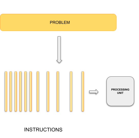
Typical programming assumes that computers execute one operation at a time in the sequence specified by your program code. At any time step, the computer’s CPU core will be working on one particular operation from the sequence. In other words, a problem is broken into discrete series of instructions that are executed one for another. Therefore only one instruction can execute at any moment in time. We will call this traditional style of sequential computing.

In contrast, with parallel computing we will now be dealing with multiple CPU cores that each are independently and simultaneously working on a series of instructions. This can allow us to do much more at once, and therefore get results more quickly than if only running an equivalent sequential program. The act of changing sequential code to parallel code is called parallelisation.

Sequential Computing

Parallel Computing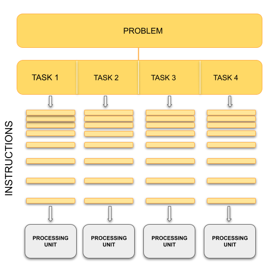

Analogy

The basic concept of parallel computing is simple to understand: we divide our job in tasks that can be executed at the same time so that we finish the job in a fraction of the time that it would have taken if the tasks are executed one by one.

Suppose that we want to paint the four walls in a room. This is our problem. We can divide our problem in 4 different tasks: paint each of the walls. In principle, our 4 tasks are independent from each other in the sense that we don’t need to finish one to start another. However, this does not mean that the tasks can be executed simultaneously or in parallel. It all depends on on the amount of resources that we have for the tasks.

If there is only one painter, they could work for a while in one wall, then start painting another one, then work a little bit on the third one, and so on. The tasks are being executed concurrently but not in parallel and only one task is being performed at a time. If we have 2 or more painters for the job, then the tasks can be performed in parallel.

Key idea

In our analogy, the painters represent CPU cores in the computers. The number of CPU cores available determines the maximum number of tasks that can be performed in parallel. The number of concurrent tasks that can be started at the same time, however is unlimited.

Parallel Programming and Memory: Processes, Threads and Memory Models

Splitting the problem into computational tasks across different processors and running them all at once may conceptually seem like a straightforward solution to achieve the desired speed-up in problem-solving. However, in practice, parallel programming involves more than just task division and introduces various complexities and considerations.

Let’s consider a scenario where you have a single CPU core, associated RAM (primary memory for faster data access), hard disk (secondary memory for slower data access), input devices (keyboard, mouse), and output devices (screen).

Now, imagine having two or more CPU cores. Suddenly, you have several new factors to take into account:

1. If there are two cores, there are two possibilities: either these cores share the same RAM (shared memory) or each core has its own dedicated RAM (private memory).
2. In the case of shared memory, what happens when two cores try to write to the same location simultaneously? This can lead to a race condition, which requires careful handling by the programmer to avoid conflicts.
3. How do we divide and distribute the computational tasks among these cores? Ensuring a balanced workload distribution is essential for optimal performance.
4. Communication between cores becomes a crucial consideration. How will the cores exchange data and synchronize their operations? Effective communication mechanisms must be established.
5. After completing the tasks, where should the final results be stored? Should they reside in the storage of Core 1, Core 2, or a central storage accessible to both? Additionally, which core is responsible for displaying output on the screen?

These considerations highlight the interplay between parallel programming and memory. To efficiently utilize multiple CPU cores, we need to understand the concepts of processes and threads, as well as different memory models—shared memory and distributed memory. These concepts form the foundation of parallel computing and play a crucial role in achieving optimal parallel execution.

To address the challenges that arise when parallelising programs across multiple cores and achieve efficient use of available resources, parallel programming frameworks like MPI and OpenMP (Open Multi-Processing) come into play. These frameworks provide tools, libraries, and methodologies to handle memory management, workload distribution, communication, and synchronization in parallel environments.

Now, let’s take a brief look at these fundamental concepts and explore the differences between MPI and OpenMP, setting the stage for a deeper understanding of MPI in the upcoming episodes

Processes

A process refers to an individual running instance of a software program. Each process operates independently and possesses its own set of resources, such as memory space and open files. As a result, data within one process remains isolated and cannot be directly accessed by other processes.

In parallel programming, the objective is to achieve parallel execution by simultaneously running coordinated processes. This naturally introduces the need for communication and data sharing among them. To facilitate this, parallel programming models like MPI come into effect. MPI provides a comprehensive set of libraries, tools, and methodologies that enable processes to exchange messages, coordinate actions, and share data, enabling parallel execution across a cluster or network of machines.

Threads

A thread is an execution unit that is part of a process. It operates within the context of a process and shares the process’s resources. Unlike processes, multiple threads within a process can access and share the same data, enabling more efficient and faster parallel programming.

Threads are lightweight and can be managed independently by a scheduler. They are units of execution in concurrent programming, allowing multiple threads to execute at the same time, making use of available CPU cores for parallel processing. Threads can improve application performance by utilizing parallelism and allowing tasks to be executed concurrently.

One advantage of using threads is that they can be easier to work with compared to processes when it comes to parallel programming. When incorporating threads, especially with frameworks like OpenMP, modifying a program becomes simpler. This ease of use stems from the fact that threads operate within the same process and can directly access shared data, eliminating the need for complex inter-process communication mechanisms required by MPI. However, it’s important to note that threads within a process are limited to a single computer. While they provide an effective means of utilizing multiple CPU cores on a single machine, they cannot extend beyond the boundaries of that computer.

Analogy

Let’s go back to our painting 4 walls analogy. Our example painters have two arms, and could potentially paint with both arms at the same time. Technically, the work being done by each arm is the work of a single painter. In this example, each painter would be a “process” (an individual instance of a program). The painters’ arms represent a “thread” of a program. Threads are separate points of execution within a single program, and can be executed either synchronously or asynchronously.

Shared vs Distributed Memory

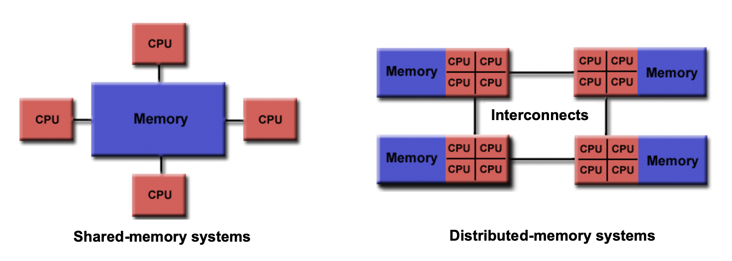
Shared memory refers to a memory model where multiple processors can directly access and modify the same memory space. Changes made by one processor are immediately visible to all other processors. Shared memory programming models, like OpenMP, simplify parallel programming by providing mechanisms for sharing and synchronizing data.

Distributed memory, on the other hand, involves memory resources that are physically separated across different computers or nodes in a network. Each processor has its own private memory, and explicit communication is required to exchange data between processors. Distributed memory programming models, such as MPI, facilitate communication and synchronization in this memory model.

Differences/Advantages/Disadvantages of Shared and Distributed Memory

• Accessibility: Shared memory allows direct access to the same memory space by all processors, while distributed memory requires explicit communication for data exchange between processors.
• Memory Scope: Shared memory provides a global memory space, enabling easy data sharing and synchronization. In distributed memory, each processor has its own private memory space, requiring explicit communication for data sharing.
• Memory Consistency: Shared memory ensures immediate visibility of changes made by one processor to all other processors. Distributed memory requires explicit communication and synchronization to maintain data consistency across processors.
• Scalability: Shared memory systems are typically limited to a single computer or node, whereas distributed memory systems can scale to larger configurations with multiple computers and nodes.
• Programming Complexity: Shared memory programming models offer simpler constructs and require less explicit communication compared to distributed memory models. Distributed memory programming involves explicit data communication and synchronization, adding complexity to the programming process.

Analogy

Imagine that all workers have to obtain their paint form a central dispenser located at the middle of the room. If each worker is using a different colour, then they can work asynchronously. However, if they use the same colour, and two of them run out of paint at the same time, then they have to synchronise to use the dispenser — one should wait while the other is being serviced.

Now let’s assume that we have 4 paint dispensers, one for each worker. In this scenario, each worker can complete their task totally on their own. They don’t even have to be in the same room, they could be painting walls of different rooms in the house, in different houses in the city, and different cities in the country. We need, however, a communication system in place. Suppose that worker A, for some reason, needs a colour that is only available in the dispenser of worker B, they must then synchronise: worker A must request the paint of worker B and worker B must respond by sending the required colour.

Key Idea

In our analogy, the paint dispenser represents access to the memory in your computer. Depending on how a program is written, access to data in memory can be synchronous or asynchronous. For the different dispensers case for your workers, however, think of the memory distributed on each node/computer of a cluster.

MPI vs OpenMP: What is the difference?

MPI	OpenMP
Defines an API, vendors provide an optimized (usually binary) library implementation that is linked using your choice of compiler.	OpenMP is integrated into the compiler (e.g., gcc) and does not offer much flexibility in terms of changing compilers or operating systems unless there is an OpenMP compiler available for the specific platform.
Offers support for C, Fortran, and other languages, making it relatively easy to port code by developing a wrapper API interface for a pre-compiled MPI implementation in a different language.	Primarily supports C, C++, and Fortran, with limited options for other programming languages.
Suitable for both distributed memory and shared memory (e.g., SMP) systems, allowing for parallelization across multiple nodes.	Designed for shared memory systems and cannot be used for parallelization across multiple computers.
Enables parallelism through both processes and threads, providing flexibility for different parallel programming approaches.	Focuses solely on thread-based parallelism, limiting its scope to shared memory environments.
Creation of process/thread instances and communication can result in higher costs and overhead.	Offers lower overhead, as inter-process communication is handled through shared memory, reducing the need for expensive process/thread creation.

Parallel Paradigms

Thinking back to shared vs distributed memory models, how to achieve a parallel computation is divided roughly into two paradigms. Let’s set both of these in context:

1. In a shared memory model, a data parallelism paradigm is typically used, as employed by OpenMP: the same operations are performed simultaneously on data that is shared across each parallel operation. Parallelism is achieved by how much of the data a single operation can act on.
2. In a distributed memory model, a message passing paradigm is used, as employed by MPI: each CPU (or core) runs an independent program. Parallelism is achieved by receiving data which it doesn’t have, conducting some operations on this data, and sending data which it has.

This division is mainly due to historical development of parallel architectures: the first one follows from shared memory architecture like SMP (Shared Memory Processors) and the second from distributed computer architecture. A familiar example of the shared memory architecture is GPU (or multi-core CPU) architecture, and an example of the distributed computing architecture is a cluster of distributed computers. Which architecture is more useful depends on what kind of problems you have. Sometimes, one has to use both!

Consider a simple loop which can be sped up if we have many cores for illustration:

for(i=0; i<N; i++) {
  a[i] = b[i] + c[i];
}

If we have N or more cores, each element of the loop can be computed in just one step (for a factor of \(N\) speed-up). Let’s look into both paradigms in a little more detail, and focus on key characteristics.

1. Data Parallelism Paradigm

One standard method for programming using data parallelism is called “OpenMP” (for “Open MultiProcessing”). To understand what data parallelism means, let’s consider the following bit of OpenMP code which parallelizes the above loop:

#pragma omp parallel for
for(i=0; i<N; i++) {
  a[i] = b[i] + c[i];
}

Parallelization achieved by just one additional line, #pragma omp parallel for, handled by the preprocessor in the compile stage, where the compiler “calculates” the data address off-set for each core and lets each one compute on a part of the whole data. This approach provides a convenient abstraction, and hides the underlying parallelisation mechanisms.

Here, the catch word is shared memory which allows all cores to access all the address space. We’ll be looking into OpenMP later in this course. In Python, process-based parallelism is supported by the multiprocessing module.

2. Message Passing Paradigm

In the message passing paradigm, each processor runs its own program and works on its own data. To work on the same problem in parallel, they communicate by sending messages to each other. Again using the above example, each core runs the same program over a portion of the data. For example, using this paradigm to parallelise the above loop instead:

for(i=0; i<m; i++) {
  a[i] = b[i] + c[i];
}

• Other than changing the number of loops from N to m, the code is exactly the same.
• m is the reduced number of loops each core needs to do (if there are N cores, m is 1 (= N/N)). But the parallelization by message passing is not complete yet. In the message passing paradigm, each core operates independently from the other cores. So each core needs to be sent the correct data to compute, which then returns the output from that computation. However, we also need a core to coordinate the splitting up of that data, send portions of that data to other cores, and to receive the resulting computations from those cores.

Summary

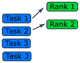
In the end, both data parallelism and message passing logically achieve the following:

Therefore, each rank essentially operates on its own set of data, regardless of paradigm. In some cases, there are advantages to combining data parallelism and message passing methods together, e.g. when there are problems larger than one GPU can handle. In this case, data parallelism is used for the portion of the problem contained within one GPU, and then message passing is used to employ several GPUs (each GPU handles a part of the problem) unless special hardware/software supports multiple GPU usage.

Algorithm Design

Designing a parallel algorithm that determines which of the two paradigms above one should follow rests on the actual understanding of how the problem can be solved in parallel. This requires some thought and practice.

To get used to “thinking in parallel”, we discuss “Embarrassingly Parallel” (EP) problems first and then we consider problems which are not EP problems.

Embarrassingly Parallel Problems

Problems which can be parallelized most easily are EP problems, which occur in many Monte Carlo simulation problems and in many big database search problems. In Monte Carlo simulations, random initial conditions are used in order to sample a real situation. So, a random number is given and the computation follows using this random number. Depending on the random number, some computation may finish quicker and some computation may take longer to finish. And we need to sample a lot (like a billion times) to get a rough picture of the real situation. The problem becomes running the same code with a different random number over and over again! In big database searches, one needs to dig through all the data to find wanted data. There may be just one datum or many data which fit the search criterion. Sometimes, we don’t need all the data which satisfies the condition. Sometimes, we do need all of them. To speed up the search, the big database is divided into smaller databases, and each smaller databases are searched independently by many workers!

Queue Method

Each worker will get tasks from a predefined queue (a random number in a Monte Carlo problem and smaller databases in a big database search problem). The tasks can be very different and take different amounts of time, but when a worker has completed its tasks, it will pick the next one from the queue.

In an MPI code, the queue approach requires the ranks to communicate what they are doing to all the other ranks, resulting in some communication overhead (but negligible compared to overall task time).

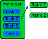
Manager / Worker Method

The manager / worker approach is a more flexible version of the queue method. We hire a manager to distribute tasks to the workers. The manager can run some complicated logic to decide which tasks to give to a worker. The manager can also perform any serial parts of the program like generating random numbers or dividing up the big database. The manager can become one of the workers after finishing managerial work.

In an MPI implementation, the main function will usually contain an if statement that determines whether the rank is the manager or a worker. The manager can execute a completely different code from the workers, or the manager can execute the same partial code as the workers once the managerial part of the code is done. It depends on whether the managerial load takes a lot of time to finish or not. Idling is a waste in parallel computing!

Because every worker rank needs to communicate with the manager, the bandwidth of the manager rank can become a bottleneck if administrative work needs a lot of information (as we can observe in real life). This can happen if the manager needs to send smaller databases (divided from one big database) to the worker ranks. This is a waste of resources and is not a suitable solution for an EP problem. Instead, it’s better to have a parallel file system so that each worker rank can access the necessary part of the big database independently.

General Parallel Problems (Non-EP Problems)

In general not all the parts of a serial code can be parallelized. So, one needs to identify which part of a serial code is parallelizable. In science and technology, many numerical computations can be defined on a regular structured data (e.g., partial differential equations in a 3D space using a finite difference method). In this case, one needs to consider how to decompose the domain so that many cores can work in parallel.

Domain Decomposition

When the data is structured in a regular way, such as when simulating atoms in a crystal, it makes sense to divide the space into domains. Each rank will handle the simulation within its own domain.

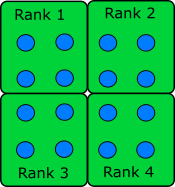
Many algorithms involve multiplying very large matrices. These include finite element methods for computational field theories as well as training and applying neural networks. The most common parallel algorithm for matrix multiplication divides the input matrices into smaller submatrices and composes the result from multiplications of the submatrices. If there are four ranks, the matrix is divided into four submatrices.

\[A = \left[ \begin{array}{cc}A_{11} & A_{12} \\ A_{21} & A_{22}\end{array} \right]\] \[B = \left[ \begin{array}{cc}B_{11} & B_{12} \\ B_{21} & B_{22}\end{array} \right]\] \[A \cdot B = \left[ \begin{array}{cc}A_{11} \cdot B_{11} + A_{12} \cdot B_{21} & A_{11} \cdot B_{12} + A_{12} \cdot B_{22} \\ A_{21} \cdot B_{11} + A_{22} \cdot B_{21} & A_{21} \cdot B_{12} + A_{22} \cdot B_{22}\end{array} \right]\]

If the number of ranks is higher, each rank needs data from one row and one column to complete its operation.

Load Balancing

Even if the data is structured in a regular way and the domain is decomposed such that each core can take charge of roughly equal amounts of the sub-domain, the work that each core has to do may not be equal. For example, in weather forecasting, the 3D spatial domain can be decomposed in an equal portion. But when the sun moves across the domain, the amount of work is different in that domain since more complicated chemistry/physics is happening in that domain. Balancing this type of loads is a difficult problem and requires a careful thought before designing a parallel algorithm.

Serial and Parallel Regions

Identify the serial and parallel regions in the following algorithm:

 vector_1[0] = 1;
 vector_1[1] = 1;
 for i in 2 ... 1000
   vector_1[i] = vector_1[i-1] + vector_1[i-2];

 for i in 0 ... 1000
   vector_2[i] = i;

 for i in 0 ... 1000
   vector_3[i] = vector_2[i] + vector_1[i];
   print("The sum of the vectors is.", vector_3[i]);

Solution

First Loop: Each iteration depends on the results of the previous two iterations in vector_1. So it is not parallelisable within itself.

Second Loop: Each iteration is independent and can be parallelised.

Third loop: Each iteration is independent within itself. While there are dependencies on vector_2[i] and vector_1[i], these dependencies are local to each iteration. This independence allows for the potential parallelization of the third loop by overlapping its execution with the second loop, assuming the results of the first loop are available or can be made available dynamically.

serial   | vector_0[0] = 1;
         | vector_1[1] = 1;
         | for i in 2 ... 1000
         |   vector_1[i] = vector_1[i-1] + vector_1[i-2];

parallel | for i in 0 ... 1000
         |   vector_2[i] = i;

parallel | for i in 0 ... 1000
         |   vector_3[i] = vector_2[i] + vector_1[i];
         |   print("The sum of the vectors is.", vector_3[i]);

The first and the second loop could also run at the same time.

Key Points

• Processes do not share memory and can reside on the same or different computers.

• Threads share memory and reside in a process on the same computer.

• MPI is an example of multiprocess programming whereas OpenMP is an example of multithreaded programming.

• Algorithms can have both parallelisable and non-parallelisable sections.

• There are two major parallelisation paradigms; data parallelism and message passing.

• MPI implements the Message Passing paradigm, and OpenMP implements data parallelism.