Porting Serial Code to MPI

Overview

Teaching: 0 min
Exercises: 0 min

Questions

What is the best way to write a parallel code?

How do I parallelise my existing serial code?

Objectives

Practice how to identify which parts of a codebase would benefit from parallelisation, and those that need to be done serially or only once

Convert a serial code into a parallel code

Differentiate between choices of communication pattern and algorithm design

In this section we will look at converting a complete code from serial to parallel in a number of steps.

An Example Iterative Poisson Solver

This episode is based on a code that solves the Poisson’s equation using an iterative method. Poisson’s equation appears in almost every field in physics, and is frequently used to model many physical phenomena such as heat conduction, and applications of this equation exist for both two and three dimensions. In this case, the equation is used in a simplified form to describe how heat diffuses in a one dimensional metal stick.

In the simulation the stick is split into a given number of slices, each with its own temperature.

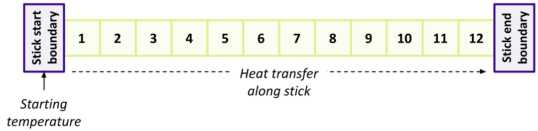
Stick divided into separate slices with touching boundaries at each end

The temperature of the stick itself across each slice is initially set to zero, whilst at one boundary of the stick the amount of heat is set to 10. The code applies steps that simulates heat transfer along it, bringing each slice of the stick closer to a solution until it reaches a desired equilibrium in temperature along the whole stick.

Let’s download the code, which can be found here, and take a look at it now.

At a High Level - main()

We’ll begin by looking at the main() function at a high level.

#define MAX_ITERATIONS 25000
#define GRIDSIZE 12

...

int main(int argc, char** argv) {

  // The heat energy in each block
  float *u, *unew, *rho;
  float h, hsq;
  double unorm, residual;
  int i;

  u = malloc(sizeof(*u) * (GRIDSIZE+2));
  unew = malloc(sizeof(*unew) * (GRIDSIZE+2));
  rho = malloc(sizeof(*rho) * (GRIDSIZE+2));

It first defines two constants that govern the scale of the simulation:

MAX_ITERATIONS: determines the maximum number of iterative steps the code will attempt in order to find a solution with sufficiently low equilibrium
GRIDSIZE: the number of slices within our stick that will be simulated. Increasing this will increase the number of stick slices to simulate, which increases the processing required

Next, it declares some arrays used during the iterative calculations:

u: each value represents the current temperature of a slice in the stick
unew: during an iterative step, is used to hold the newly calculated temperature of a slice in the stick
rho: holds a separate coefficient for each slice of the stick, used as part of the iterative calculation to represent potentially different boundary conditions for each stick slice. For simplicity, we’ll assume completely homogeneous boundary conditions, so these potentials are zero

Note we are defining each of our array sizes with two additional elements, the first of which represents a touching ‘boundary’ before the stick, i.e. something with a potentially different temperature touching the stick. The second added element is at the end of the stick, representing a similar boundary at the opposite end.

The next step is to initialise the initial conditions of the simulation:

  // Set up parameters
  h = 0.1;
  hsq = h*h;
  residual = 1e-5;

  // Initialise the u and rho field to 0
  for (i = 0; i <= GRIDSIZE+1; i++) {
    u[i] = 0.0;
    rho[i] = 0.0;
  }

  // Create a start configuration with the heat energy
  // u=10 at the x=0 boundary for rank 1
  u[0] = 10.0;

residual here refers to the threshold of temperature equilibrium along the stick we wish to achieve. Once it’s within this threshold, the simulation will end. Note that initially, u is set entirely to zero, representing a temperature of zero along the length of the stick. As noted, rho is set to zero here for simplicity.

Remember that additional first element of u? Here we set it to a temperature of 10.0 to represent something with that temperature touching the stick at one end, to initiate the process of heat transfer we wish to simulate.

Next, the code iteratively calls poisson_step() to calculate the next set of results, until either the maximum number of steps is reached, or a particular measure of the difference in temperature along the stick returned from this function (unorm) is below a particular threshold.

  // Run iterations until the field reaches an equilibrium
  // and no longer changes
  for (i = 0; i < NUM_ITERATIONS; i++) {
    unorm = poisson_step(u, unew, rho, hsq, GRIDSIZE);
    if (sqrt(unorm) < sqrt(residual)) break;
  }

Finally, just for show, the code outputs a representation of the result - the end temperature of each slice of the stick.

  printf("Final result:\n");
  for (int j = 1; j <= GRIDSIZE; j++) {
    printf("%d-", (int) u[j]);
  }
  printf("\n");
  printf("Run completed in %d iterations with residue %g\n", i, unorm);
}

The Iterative Function - poisson_step()

The poisson_step() progresses the simulation by a single step. After it accepts its arguments, for each slice in the stick it calculates a new value based on the temperatures of its neighbours:

  for (int i = 1; i <= points; i++) {
     float difference = u[i-1] + u[i+1];
     unew[i] = 0.5 * (difference - hsq*rho[i]);
  }

Next, it calculates a value representing the overall cumulative change in temperature along the stick compared to its previous state, which as we saw before, is used to determine if we’ve reached a stable equilibrium and may exit the simulation:

  unorm = 0.0;
  for (int i = 1;i <= points; i++) {
     float diff = unew[i]-u[i];
     unorm += diff*diff;
  }

And finally, the state of the stick is set to the newly calculated values, and unorm is returned from the function:

  // Overwrite u with the new field
  for (int i = 1;i <= points;i++) {
     u[i] = unew[i];
  }

  return unorm;
}

Compiling and Running the Poisson Code

You may compile and run the code as follows:

gcc poisson.c -o poisson -lm
./poisson

And should see the following:

Final result:
9-8-7-6-6-5-4-3-3-2-1-0-
Run completed in 182 iterations with residue 9.60328e-06

Here, we can see a basic representation of the temperature of each slice of the stick at the end of the simulation, and how the initial 10.0 temperature applied at the beginning of the stick has transferred along it to this final state. Ordinarily, we might output the full sequence to a file, but we’ve simplified it for convenience here.

Approaching Parallelism

So how should we make use of an MPI approach to parallelise this code? A good place to start is to consider the nature of the data within this computation, and what we need to achieve.

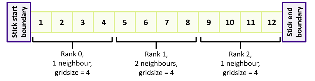
For a number of iterative steps, currently the code computes the next set of values for the entire stick. So at a high level one approach using MPI would be to split this computation by dividing the stick into sections each with a number of slices, and have a separate rank responsible for computing iterations for those slices within its given section. Essentially then, for simplicity we may consider each section a stick on its own, with either two neighbours at touching boundaries (for middle sections of the stick), or one touching boundary neighbour (for sections at the beginning and end of the stick, which also have either a start or end stick boundary touching them). For example, considering a GRIDSIZE of 12 and three ranks:

Stick divisions subdivided across ranks

We might also consider subdividing the number of iterations, and parallelise across these instead. However, this is far less compelling since each step is completely dependent on the results of the prior step, so by its nature steps must be done serially.

The next step is to consider in more detail this approach to parallelism with our code.

Parallelism and Data Exchange

Looking at the code, which parts would benefit most from parallelisation, and are there any regions that require data exchange across its processes in order for the simulation to work as we intend?

Solution

Potentially, the following regions could be executed in parallel:

The setup, when initialising the fields

The calculation of each time step, unew - this is the most computationally intensive of the loops

Calculation of the cumulative temperature difference, unorm

Overwriting the field u with the result of the new calculation

As GRIDSIZE is increased, these will take proportionally more time to complete, so may benefit from parallelisation.

However, there are a few regions in the code that will require exchange of data across the parallel executions to work correctly:

Calculation of unorm is a sum that requires difference data from all sections of the stick, so we’d need to somehow communicate these difference values to a single rank that computes and receives the overall sum

Each section of the stick does not compute a single step in isolation, it needs boundary data from neighbouring sections of the stick to arrive at its computed temperature value for that step, so we’d need to communicate temperature values between neighbours (i.e. using a nearest neighbours communication pattern)

We also need to identify any sizeable serial regions. The sum of the serial regions gives the minimum amount of time it will take to run the program. If the serial parts are a significant part of the algorithm, it may not be possible to write an efficient parallel version.

Serial Regions

Examine the code and try to identify any serial regions that can’t (or shouldn’t) be parallelised.

Solution

There aren’t any large or time consuming serial regions, which is good from a parallelism perspective. However, there are a couple of small regions that are not amenable to running in parallel:

Setting the 10.0 initial temperature condition at the stick ‘starting’ boundary. We only need to set this once at the beginning of the stick, and not at the boundary of every section of the stick

Printing a representation of the final result, since this only needs to be done once to represent the whole stick, and not for every section.

So we’d need to ensure only one rank deals with these, which in MPI is typically the zeroth rank. This also makes sense in terms of our parallelism approach, since the zeroth rank would be the beginning of the stick, where we’d set the initial boundary temperature.

Parallelising our Code

So now let’s apply what we’ve learned about MPI together with our consideration of the code. First, make a copy of the poisson.c code that we will work on (don’t modify the original, we’ll need this later!). In the shell, for example:

cp poisson.c poisson_mpi.c

And then we can add our MPI parallelisation modifications to poisson_mpi.c

We’ll start at a high level with main(), although first add #include <mpi.h> at the top of our code so we can make use of MPI. We’ll do this parallelisation in a number of stages.

In MPI, all ranks execute the same code. When writing a parallel code with MPI, a good place to start is to think about a single rank. What does this rank need to do, and what information does it need to do it?

The first goal should be to write a simple code that works correctly. We can always optimise further later!

main(): Adding MPI at a High-level

Then as we usually do, let’s initialise MPI and obtain our rank and total number of ranks. With the latter information, we can then calculate how many slices of the stick this rank will compute. Near the top of main() add the following:

  int rank, n_ranks, rank_gridsize;

  MPI_Init(&argc, &argv);

  // Find the number of slices calculated by each rank
  // The simple calculation here assumes that GRIDSIZE is divisible by n_ranks
  MPI_Comm_rank(MPI_COMM_WORLD, &rank);
  MPI_Comm_size(MPI_COMM_WORLD, &n_ranks);
  rank_gridsize = GRIDSIZE / n_ranks;

Using rank_gridsize, we can now amend our initial array declaration sizes to use this instead:

  u = malloc(sizeof(*u) * (rank_gridsize + 2));
  unew = malloc(sizeof(*unew) * (rank_gridsize + 2));
  rho = malloc(sizeof(*rho) * (rank_gridsize + 2));

Then at the very end of main() let’s complete our use of MPI:

  MPI_Finalize();
}

main(): Initialising the Simulation and Printing the Result

Since we’re not initialising for the entire stick (GRIDSIZE) but just the section apportioned to our rank (rank_gridsize), we need to amend the loop that initialises u and rho accordingly, to:

  // Initialise the u and rho field to 0
  for (i = 0; i <= rank_gridsize+1; i++) {
    u[i] = 0.0;
    rho[i] = 0.0;
  }

As we found out in the Serial Regions exercise, we need to ensure that only a single rank (rank zero) needs to initiate the starting temperature within it’s section, so we need to put a condition on that initialisation:

  // Create a start configuration with the heat energy
  // u=10 at the x=0 boundary for rank 0
  if (rank == 0)
    u[0] = 10.0;

We also need to collect the overall results from all ranks and output that collected result, but again, only for rank zero. To collect the results from all ranks (held in u) we can use MPI_Gather(), to send all u results to rank zero to hold in a results array. Note that this will also include the result from rank zero!

Add the following to the list of declarations at the start of main():

  float *resultbuf;

Then before MPI_Finalize() let’s amend the code to the following:

  // Gather results from all ranks
  // We need to send data starting from the second element of u, since u[0] is a boundary
  resultbuf = malloc(sizeof(*resultbuf) * GRIDSIZE);
  MPI_Gather(&u[1], rank_gridsize, MPI_FLOAT, resultbuf, rank_gridsize, MPI_FLOAT, 0, MPI_COMM_WORLD);
  
  if (rank == 0) {
    printf("Final result:\n");
    for (int j = 0; j < GRIDSIZE; j++) {
      printf("%d-", (int) resultbuf[j]);
    }
    printf("\nRun completed in %d iterations with residue %g\n", i, unorm);
  }

MPI_Gather() is ideally suited for our purposes, since results from ranks are arranged within resultbuf in rank order, so we end up with all slices across all ranks representing the entire stick. However, note that we need to send our data starting from u[1], since u[0] is the section’s boundary value we don’t want to include.

This has an interesting effect we need to account for - note the change to the for loop. Since we are gathering data from each rank (including rank 0) starting from u[1], resultbuf will not contain any section boundary values so our loop no longer needs to skip the first value.

main(): Invoking the Step Function

Before we parallelise the poisson_step() function, let’s amend how we invoke it and pass it some additional parameters it will need. We need to amend how many slices it will compute, and add the rank and n_ranks variables, since we know from Parallelism and Data Exchange that it will need to perform some data exchange with other ranks:

    unorm = poisson_step(u, unew, rho, hsq, rank_gridsize, rank, n_ranks );

poisson_step(): Updating our Function Definition

Moving into the poisson_step() function, we first amend our function to include the changes to parameters:

double poisson_step(
  float *u, float *unew, float *rho,
  float hsq, int points,
  int rank, int n_ranks
) {

poisson_step(): Calculating a Global `unorm`

We know from Parallelism and Data Exchange that we need to calculate unorm across all ranks. We already have it calculated for separate ranks, so need to reduce those values in an MPI sense to a single summed value. For this, we can use MPI_Allreduce().

Insert the following into the poisson_step() function, putting the declarations at the top of the function, and the MPI_Allreduce() after the calculation of unorm:

  double unorm, global_unorm;
  
  MPI_Allreduce(&unorm, &global_unorm, 1, MPI_DOUBLE, MPI_SUM, MPI_COMM_WORLD);

So here, we use this function in an MPI_SUM mode, which will sum all instances of unorm and place the result in a single (1) value global_unorm`. We must also remember to amend the return value to this global version, since we need to calculate equilibrium across the entire stick:

  return global_unorm;
}

poisson_step(): Communicate Boundaries to Neighbours

In order for our parallel code to work, we know from Parallelism and Data Exchange that each section of slices is not computed in isolation. After we’ve computed new values we need to send our boundary slice values to our neighbours if those neighbours exist - the beginning and end of the stick will each only have one neighbour, so we need to account for that.

We also need to ensure that we don’t encounter a deadlock situation when exchanging the data between neighbours. They can’t all send to the rightmost neighbour simultaneously, since none will then be waiting and able to receive. We need a message exchange strategy here, so let’s have all odd-numbered ranks send their data first (to be received by even ranks), then have our even ranks send their data (to be received by odd ranks). Such an order might look like this (highlighting the odd ranks - only one in this example - with the order of communications indicated numerically):

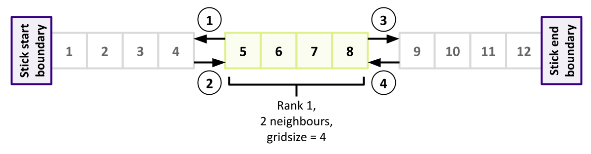
Communication strategy - odd ranks send to potential neighbours first, then receive from them

So following the MPI_Allreduce() we’ve just added, let’s deal with odd ranks first (again, put the declarations at the top of the function):

  float sendbuf, recvbuf;
  MPI_Status mpi_status;

  // The u field has been changed, communicate it to neighbours
  // With blocking communication, half the ranks should send first
  // and the other half should receive first
  if ((rank%2) == 1) {
    // Ranks with odd number send first

    // Send data down from rank to rank-1
    sendbuf = unew[1];
    MPI_Send(&sendbuf, 1, MPI_FLOAT, rank-1, 1, MPI_COMM_WORLD);
    // Receive dat from rank-1
    MPI_Recv(&recvbuf, 1, MPI_FLOAT, rank-1, 2, MPI_COMM_WORLD, &mpi_status);
    u[0] = recvbuf;

    if (rank != (n_ranks-1)) {
      // Send data up to rank+1 (if I'm not the last rank)
      MPI_Send(&u[points], 1, MPI_FLOAT, rank+1, 1, MPI_COMM_WORLD);
      // Receive data from rank+1
      MPI_Recv(&u[points+1], 1, MPI_FLOAT, rank+1, 2, MPI_COMM_WORLD, &mpi_status);
    }

Here we use C’s inbuilt modulus operator (%) to determine if the rank is odd. If so, we exchange some data with the rank preceding us, and the one following.

We first send our newly computed leftmost value (at position 1 in our array) to the rank preceding us. Since we’re an odd rank, we can always assume a rank preceding us exists, since the earliest odd rank 1 will exchange with rank 0. Then, we receive the rightmost boundary value from that rank.

Then, if the rank following us exists, we do the same, but this time we send the rightmost value at the end of our stick section, and receive the corresponding value from that rank.

These exchanges mean that - as an odd rank - we now have effectively exchanged the states of the start and end of our slices with our respective neighbours.

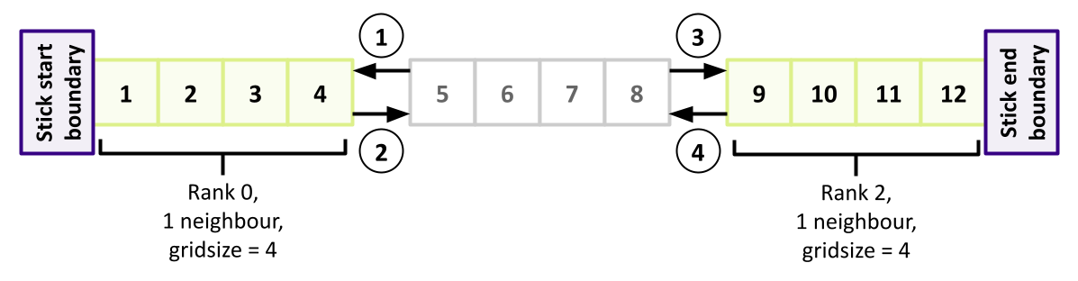
And now we need to do the same for those neighbours (the even ranks), mirroring the same communication pattern but in the opposite order of receive/send. From the perspective of evens, it should look like the following (highlighting the two even ranks):

Communication strategy - even ranks first receive from odd ranks, then send to them

  } else {
    // Ranks with even number receive first

    if (rank != 0) {
      // Receive data from rank-1 (if I'm not the first rank)
      MPI_Recv(&u[0], 1, MPI_FLOAT, rank-1, 1, MPI_COMM_WORLD, &mpi_status);
      // Send data down to rank-1
      MPI_Send(&u[1], 1, MPI_FLOAT, rank-1, 2, MPI_COMM_WORLD);
    }

    if (rank != (n_ranks-1)) {
      // Receive data from rank+1 (if I'm not the last rank)
      MPI_Recv(&u[points+1], 1, MPI_FLOAT, rank+1, 1, MPI_COMM_WORLD, &mpi_status);
      // Send data up to rank+1
      MPI_Send(&u[points], 1, MPI_FLOAT, rank+1, 2, MPI_COMM_WORLD);
    }
  }

Once complete across all ranks, every rank will then have the slice boundary data from its neighbours ready for the next iteration.

Running our Parallel Code

You can obtain a full version of the parallelised Poisson code from here. Now we have the parallelised code in place, we can compile and run it, e.g.:

mpicc poisson_mpi.c -o poisson_mpi -lm
mpirun -n 2 poisson_mpi

Final result:
9-8-7-6-6-5-4-3-3-2-1-0-
Run completed in 182 iterations with residue 9.60328e-06

Note that as it stands, the implementation assumes that GRIDSIZE is divisible by n_ranks. So to guarantee correct output, we should use only

Testing our Parallel Code

We should always ensure that as our parallel version is developed, that it behaves the same as our serial version. This may not be possible initially, particularly as large parts of the code need converting to use MPI, but where possible, we should continue to test. So we should test once we have an initial MPI version, and as our code develops, perhaps with new optimisations to improve performance, we should test then too.

An Initial Test

Test the mpi version of your code against the serial version, using 1, 2, 3, and 4 ranks with the MPI version. Are the results as you would expect? What happens if you test with 5 ranks, and why?

Solution

Using these ranks, the MPI results should be the same as our serial version. Using 5 ranks, our MPI version yields 9-8-7-6-5-4-3-2-1-0-0-0- which is incorrect. This is because the rank_gridsize = GRIDSIZE / n_ranks calculation becomes rank_gridsize = 12 / 5, which produces 2.4. This is then converted to the integer 2, which means each of the 5 ranks is only operating on 2 slices each, for a total of 10 slices. This doesn’t fill resultbuf with results representing an expected GRIDSIZE of 12, hence the incorrect answer.

This highlights another aspect of complexity we need to take into account when writing such parallel implementations, where we must ensure a problem space is correctly subdivided. In this case, we could implement a more careful way to subdivide the slices across the ranks, with some ranks obtaining more slices to make up the shortfall correctly.

Limitations!

You may remember that for the purposes of this episode we’ve assumed a homogeneous stick, by setting the rho coefficient to zero for every slice. As a thought experiment, if we wanted to address this limitation and model an inhomogeneous stick with different static coefficients for each slice, how could we amend our code to allow this correctly for each slice across all ranks?
Solution

One way would be to create a static lookup array with a GRIDSIZE number of elements. This could be defined in a separate .h file and imported using #include. Each rank could then read the rho values for the specific slices in its section from the array and use those. At initialisation, instead of setting it to zero we could do:
    rho[i] = rho_coefficients[(rank * rank_gridsize) + i]

Key Points

Start from a working serial code

Write a parallel implementation for each function or parallel region

Connect the parallel regions with a minimal amount of communication

Continuously compare the developing parallel code with the working serial code

previous episode

next episode

Porting Serial Code to MPI

Overview

An Example Iterative Poisson Solver

At a High Level - main()

The Iterative Function - poisson_step()

Compiling and Running the Poisson Code

Approaching Parallelism

Parallelism and Data Exchange

Solution

Serial Regions

Solution

Parallelising our Code

main(): Adding MPI at a High-level

main(): Initialising the Simulation and Printing the Result

main(): Invoking the Step Function

poisson_step(): Updating our Function Definition

poisson_step(): Calculating a Global `unorm`

poisson_step(): Communicate Boundaries to Neighbours

Running our Parallel Code

Testing our Parallel Code

An Initial Test

Solution

Limitations!

Solution

Key Points

previous episode

next episode

previous episode

next episode

Porting Serial Code to MPI

Overview

An Example Iterative Poisson Solver

At a High Level - main()

The Iterative Function - poisson_step()

Compiling and Running the Poisson Code

Approaching Parallelism

Parallelism and Data Exchange

Solution

Serial Regions

Solution

Parallelising our Code

main(): Adding MPI at a High-level

main(): Initialising the Simulation and Printing the Result

main(): Invoking the Step Function

poisson_step(): Updating our Function Definition

poisson_step(): Calculating a Global unorm

poisson_step(): Communicate Boundaries to Neighbours

Running our Parallel Code

Testing our Parallel Code

An Initial Test

Solution

Limitations!

Solution

Key Points

previous episode

next episode

poisson_step(): Calculating a Global `unorm`