Introduction to Parallelism
Overview
Teaching: 15 min
Exercises: 0 minQuestions
What is parallelisation and parallel programming?
How do MPI and OpenMP differ?
Which parts of a program are amenable to parallelisation?
How do we characterise the classes of problems to which parallelism can be applied?
How should I approach parallelising my program?
Objectives
Describe what the Message Passing Interface (MPI) is
Use the MPI API in a program
Compile and run MPI applications
Use MPI to coordinate the use of multiple processes across CPUs
Submit an MPI program to the Slurm batch scheduler
Parallel programming has been important to scientific computing for decades as a way to decrease program run times, making more complex analyses possible (e.g. climate modeling, gene sequencing, pharmaceutical development, aircraft design). During this course you will learn to design parallel algorithms and write parallel programs using the MPI library. MPI stands for Message Passing Interface, and is a low level, minimal and extremely flexible set of commands for communicating between copies of a program. Before we dive into the details of MPI, let’s first familiarize ourselves with key concepts that lay the groundwork for parallel programming.
What is Parallelisation?
At some point in your career, you’ve probably asked the question “How can I make my code run faster?”. Of course, the answer to this question will depend sensitively on your specific situation, but here are a few approaches you might try doing:
- Optimize the code.
- Move computationally demanding parts of the code from an interpreted language (Python, Ruby, etc.) to a compiled language (C/C++, Fortran, Julia, Rust, etc.).
- Use better theoretical methods that require less computation for the same accuracy.
Each of the above approaches is intended to reduce the total amount of work required by the computer to run your code. A different strategy for speeding up codes is parallelisation, in which you split the computational work among multiple processing units that labor simultaneously. The “processing units” might include central processing units (CPUs), graphics processing units (GPUs), vector processing units (VPUs), or something similar.
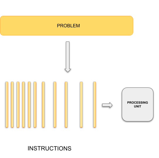
Typical programming assumes that computers execute one operation at a time in the sequence specified by your program code. At any time step, the computer’s CPU core will be working on one particular operation from the sequence. In other words, a problem is broken into discrete series of instructions that are executed one for another. Therefore only one instruction can execute at any moment in time. We will call this traditional style of sequential computing.
In contrast, with parallel computing we will now be dealing with multiple CPU cores that each are independently and simultaneously working on a series of instructions. This can allow us to do much more at once, and therefore get results more quickly than if only running an equivalent sequential program. The act of changing sequential code to parallel code is called parallelisation.
Sequential Computing
|
Parallel Computing 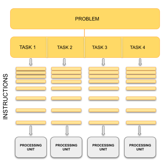
|
Analogy
The basic concept of parallel computing is simple to understand: we divide our job in tasks that can be executed at the same time so that we finish the job in a fraction of the time that it would have taken if the tasks are executed one by one.
Suppose that we want to paint the four walls in a room. This is our problem. We can divide our problem in 4 different tasks: paint each of the walls. In principle, our 4 tasks are independent from each other in the sense that we don’t need to finish one to start another. However, this does not mean that the tasks can be executed simultaneously or in parallel. It all depends on on the amount of resources that we have for the tasks.
If there is only one painter, they could work for a while in one wall, then start painting another one, then work a little bit on the third one, and so on. The tasks are being executed concurrently but not in parallel and only one task is being performed at a time. If we have 2 or more painters for the job, then the tasks can be performed in parallel.
Key idea
In our analogy, the painters represent CPU cores in the computers. The number of CPU cores available determines the maximum number of tasks that can be performed in parallel. The number of concurrent tasks that can be started at the same time, however is unlimited.
Parallel Programming and Memory: Processes, Threads and Memory Models
Splitting the problem into computational tasks across different processors and running them all at once may conceptually seem like a straightforward solution to achieve the desired speed-up in problem-solving. However, in practice, parallel programming involves more than just task division and introduces various complexities and considerations.
Let’s consider a scenario where you have a single CPU core, associated RAM (primary memory for faster data access), hard disk (secondary memory for slower data access), input devices (keyboard, mouse), and output devices (screen).
Now, imagine having two or more CPU cores. Suddenly, you have several new factors to take into account:
- If there are two cores, there are two possibilities: either these cores share the same RAM (shared memory) or each core has its own dedicated RAM (private memory).
- In the case of shared memory, what happens when two cores try to write to the same location simultaneously? This can lead to a race condition, which requires careful handling by the programmer to avoid conflicts.
- How do we divide and distribute the computational tasks among these cores? Ensuring a balanced workload distribution is essential for optimal performance.
- Communication between cores becomes a crucial consideration. How will the cores exchange data and synchronize their operations? Effective communication mechanisms must be established.
- After completing the tasks, where should the final results be stored? Should they reside in the storage of Core 1, Core 2, or a central storage accessible to both? Additionally, which core is responsible for displaying output on the screen?
These considerations highlight the interplay between parallel programming and memory. To efficiently utilize multiple CPU cores, we need to understand the concepts of processes and threads, as well as different memory models—shared memory and distributed memory. These concepts form the foundation of parallel computing and play a crucial role in achieving optimal parallel execution.
To address the challenges that arise when parallelising programs across multiple cores and achieve efficient use of available resources, parallel programming frameworks like MPI and OpenMP (Open Multi-Processing) come into play. These frameworks provide tools, libraries, and methodologies to handle memory management, workload distribution, communication, and synchronization in parallel environments.
Now, let’s take a brief look at these fundamental concepts and explore the differences between MPI and OpenMP, setting the stage for a deeper understanding of MPI in the upcoming episodes
Processes
A process refers to an individual running instance of a software program. Each process operates independently and possesses its own set of resources, such as memory space and open files. As a result, data within one process remains isolated and cannot be directly accessed by other processes.
In parallel programming, the objective is to achieve parallel execution by simultaneously running coordinated processes. This naturally introduces the need for communication and data sharing among them. To facilitate this, parallel programming models like MPI come into effect. MPI provides a comprehensive set of libraries, tools, and methodologies that enable processes to exchange messages, coordinate actions, and share data, enabling parallel execution across a cluster or network of machines.
Threads
A thread is an execution unit that is part of a process. It operates within the context of a process and shares the process’s resources. Unlike processes, multiple threads within a process can access and share the same data, enabling more efficient and faster parallel programming.
Threads are lightweight and can be managed independently by a scheduler. They are units of execution in concurrent programming, allowing multiple threads to execute at the same time, making use of available CPU cores for parallel processing. Threads can improve application performance by utilizing parallelism and allowing tasks to be executed concurrently.
One advantage of using threads is that they can be easier to work with compared to processes when it comes to parallel programming. When incorporating threads, especially with frameworks like OpenMP, modifying a program becomes simpler. This ease of use stems from the fact that threads operate within the same process and can directly access shared data, eliminating the need for complex inter-process communication mechanisms required by MPI. However, it’s important to note that threads within a process are limited to a single computer. While they provide an effective means of utilizing multiple CPU cores on a single machine, they cannot extend beyond the boundaries of that computer.


Analogy
Let’s go back to our painting 4 walls analogy. Our example painters have two arms, and could potentially paint with both arms at the same time. Technically, the work being done by each arm is the work of a single painter. In this example, each painter would be a “process” (an individual instance of a program). The painters’ arms represent a “thread” of a program. Threads are separate points of execution within a single program, and can be executed either synchronously or asynchronously.
Shared vs Distributed Memory
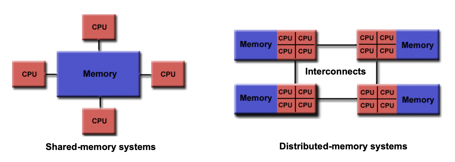
Shared memory refers to a memory model where multiple processors can directly access and modify the same memory space. Changes made by one processor are immediately visible to all other processors. Shared memory programming models, like OpenMP, simplify parallel programming by providing mechanisms for sharing and synchronizing data.
Distributed memory, on the other hand, involves memory resources that are physically separated across different computers or nodes in a network. Each processor has its own private memory, and explicit communication is required to exchange data between processors. Distributed memory programming models, such as MPI, facilitate communication and synchronization in this memory model.
Differences/Advantages/Disadvantages of Shared and Distributed Memory
- Accessibility: Shared memory allows direct access to the same memory space by all processors, while distributed memory requires explicit communication for data exchange between processors.
- Memory Scope: Shared memory provides a global memory space, enabling easy data sharing and synchronization. In distributed memory, each processor has its own private memory space, requiring explicit communication for data sharing.
- Memory Consistency: Shared memory ensures immediate visibility of changes made by one processor to all other processors. Distributed memory requires explicit communication and synchronization to maintain data consistency across processors.
- Scalability: Shared memory systems are typically limited to a single computer or node, whereas distributed memory systems can scale to larger configurations with multiple computers and nodes.
- Programming Complexity: Shared memory programming models offer simpler constructs and require less explicit communication compared to distributed memory models. Distributed memory programming involves explicit data communication and synchronization, adding complexity to the programming process.
Analogy
Imagine that all workers have to obtain their paint form a central dispenser located at the middle of the room. If each worker is using a different colour, then they can work asynchronously. However, if they use the same colour, and two of them run out of paint at the same time, then they have to synchronise to use the dispenser — one should wait while the other is being serviced.
Now let’s assume that we have 4 paint dispensers, one for each worker. In this scenario, each worker can complete their task totally on their own. They don’t even have to be in the same room, they could be painting walls of different rooms in the house, in different houses in the city, and different cities in the country. We need, however, a communication system in place. Suppose that worker A, for some reason, needs a colour that is only available in the dispenser of worker B, they must then synchronise: worker A must request the paint of worker B and worker B must respond by sending the required colour.
Key Idea
In our analogy, the paint dispenser represents access to the memory in your computer. Depending on how a program is written, access to data in memory can be synchronous or asynchronous. For the different dispensers case for your workers, however, think of the memory distributed on each node/computer of a cluster.
MPI vs OpenMP: What is the difference?
MPI OpenMP Defines an API, vendors provide an optimized (usually binary) library implementation that is linked using your choice of compiler. OpenMP is integrated into the compiler (e.g., gcc) and does not offer much flexibility in terms of changing compilers or operating systems unless there is an OpenMP compiler available for the specific platform. Offers support for C, Fortran, and other languages, making it relatively easy to port code by developing a wrapper API interface for a pre-compiled MPI implementation in a different language. Primarily supports C, C++, and Fortran, with limited options for other programming languages. Suitable for both distributed memory and shared memory (e.g., SMP) systems, allowing for parallelization across multiple nodes. Designed for shared memory systems and cannot be used for parallelization across multiple computers. Enables parallelism through both processes and threads, providing flexibility for different parallel programming approaches. Focuses solely on thread-based parallelism, limiting its scope to shared memory environments. Creation of process/thread instances and communication can result in higher costs and overhead. Offers lower overhead, as inter-process communication is handled through shared memory, reducing the need for expensive process/thread creation.
Parallel Paradigms
Thinking back to shared vs distributed memory models, how to achieve a parallel computation is divided roughly into two paradigms. Let’s set both of these in context:
- In a shared memory model, a data parallelism paradigm is typically used, as employed by OpenMP: the same operations are performed simultaneously on data that is shared across each parallel operation. Parallelism is achieved by how much of the data a single operation can act on.
- In a distributed memory model, a message passing paradigm is used, as employed by MPI: each CPU (or core) runs an independent program. Parallelism is achieved by receiving data which it doesn’t have, conducting some operations on this data, and sending data which it has.
This division is mainly due to historical development of parallel architectures: the first one follows from shared memory architecture like SMP (Shared Memory Processors) and the second from distributed computer architecture. A familiar example of the shared memory architecture is GPU (or multi-core CPU) architecture, and an example of the distributed computing architecture is a cluster of distributed computers. Which architecture is more useful depends on what kind of problems you have. Sometimes, one has to use both!
Consider a simple loop which can be sped up if we have many cores for illustration:
for (i = 0; i < N; ++i) {
  a[i] = b[i] + c[i];
}
If we have N or more cores, each element of the loop can be computed in
just one step (for a factor of \(N\) speed-up). Let’s look into both paradigms in a little more detail, and focus on key characteristics.
1. Data Parallelism Paradigm
One standard method for programming using data parallelism is called “OpenMP” (for “Open MultiProcessing”). To understand what data parallelism means, let’s consider the following bit of OpenMP code which parallelizes the above loop:
#pragma omp parallel for
for (i = 0; i < N; ++i) {
  a[i] = b[i] + c[i];
}
Parallelization achieved by just one additional line,
#pragma omp parallel for, handled by the preprocessor in the compile stage, where the compiler “calculates” the data address off-set for each core and lets each one compute on a part of the whole data. This approach provides a convenient abstraction, and hides the underlying parallelisation mechanisms.Here, the catch word is shared memory which allows all cores to access all the address space. We’ll be looking into OpenMP later in this course. In Python, process-based parallelism is supported by the multiprocessing module.
2. Message Passing Paradigm
In the message passing paradigm, each processor runs its own program and works on its own data. To work on the same problem in parallel, they communicate by sending messages to each other. Again using the above example, each core runs the same program over a portion of the data. For example, using this paradigm to parallelise the above loop instead:
for ( i = 0; i < m; ++i) {
  a[i] = b[i] + c[i];
}
- Other than changing the number of loops from
Ntom, the code is exactly the same.mis the reduced number of loops each core needs to do (if there areNcores,mis 1 (=N/N)). But the parallelization by message passing is not complete yet. In the message passing paradigm, each core operates independently from the other cores. So each core needs to be sent the correct data to compute, which then returns the output from that computation. However, we also need a core to coordinate the splitting up of that data, send portions of that data to other cores, and to receive the resulting computations from those cores.Summary
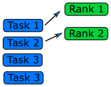
In the end, both data parallelism and message passing logically achieve the following:
Therefore, each rank essentially operates on its own set of data, regardless of paradigm. In some cases, there are advantages to combining data parallelism and message passing methods together, e.g. when there are problems larger than one GPU can handle. In this case, data parallelism is used for the portion of the problem contained within one GPU, and then message passing is used to employ several GPUs (each GPU handles a part of the problem) unless special hardware/software supports multiple GPU usage.
Algorithm Design
Designing a parallel algorithm that determines which of the two paradigms above one should follow rests on the actual understanding of how the problem can be solved in parallel. This requires some thought and practice.
To get used to “thinking in parallel”, we discuss “Embarrassingly Parallel” (EP) problems first and then we consider problems which are not EP problems.
Embarrassingly Parallel Problems
Problems which can be parallelized most easily are EP problems, which occur in many Monte Carlo simulation problems and in many big database search problems. In Monte Carlo simulations, random initial conditions are used in order to sample a real situation. So, a random number is given and the computation follows using this random number. Depending on the random number, some computation may finish quicker and some computation may take longer to finish. And we need to sample a lot (like a billion times) to get a rough picture of the real situation. The problem becomes running the same code with a different random number over and over again! In big database searches, one needs to dig through all the data to find wanted data. There may be just one datum or many data which fit the search criterion. Sometimes, we don’t need all the data which satisfies the condition. Sometimes, we do need all of them. To speed up the search, the big database is divided into smaller databases, and each smaller databases are searched independently by many workers!
Queue Method
Each worker will get tasks from a predefined queue (a random number in a Monte Carlo problem and smaller databases in a big database search problem). The tasks can be very different and take different amounts of time, but when a worker has completed its tasks, it will pick the next one from the queue.
In an MPI code, the queue approach requires the ranks to communicate what they are doing to all the other ranks, resulting in some communication overhead (but negligible compared to overall task time).
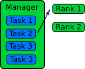
Manager / Worker Method
The manager / worker approach is a more flexible version of the queue method. We hire a manager to distribute tasks to the workers. The manager can run some complicated logic to decide which tasks to give to a worker. The manager can also perform any serial parts of the program like generating random numbers or dividing up the big database. The manager can become one of the workers after finishing managerial work.
In an MPI implementation, the main function will usually contain an
ifstatement that determines whether the rank is the manager or a worker. The manager can execute a completely different code from the workers, or the manager can execute the same partial code as the workers once the managerial part of the code is done. It depends on whether the managerial load takes a lot of time to finish or not. Idling is a waste in parallel computing!Because every worker rank needs to communicate with the manager, the bandwidth of the manager rank can become a bottleneck if administrative work needs a lot of information (as we can observe in real life). This can happen if the manager needs to send smaller databases (divided from one big database) to the worker ranks. This is a waste of resources and is not a suitable solution for an EP problem. Instead, it’s better to have a parallel file system so that each worker rank can access the necessary part of the big database independently.
General Parallel Problems (Non-EP Problems)
In general not all the parts of a serial code can be parallelized. So, one needs to identify which part of a serial code is parallelizable. In science and technology, many numerical computations can be defined on a regular structured data (e.g., partial differential equations in a 3D space using a finite difference method). In this case, one needs to consider how to decompose the domain so that many cores can work in parallel.
Domain Decomposition
When the data is structured in a regular way, such as when simulating atoms in a crystal, it makes sense to divide the space into domains. Each rank will handle the simulation within its own domain.
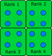
Many algorithms involve multiplying very large matrices. These include finite element methods for computational field theories as well as training and applying neural networks. The most common parallel algorithm for matrix multiplication divides the input matrices into smaller submatrices and composes the result from multiplications of the submatrices. If there are four ranks, the matrix is divided into four submatrices.
\[A = \left[ \begin{array}{cc}A_{11} & A_{12} \\ A_{21} & A_{22}\end{array} \right]\] \[B = \left[ \begin{array}{cc}B_{11} & B_{12} \\ B_{21} & B_{22}\end{array} \right]\] \[A \cdot B = \left[ \begin{array}{cc}A_{11} \cdot B_{11} + A_{12} \cdot B_{21} & A_{11} \cdot B_{12} + A_{12} \cdot B_{22} \\ A_{21} \cdot B_{11} + A_{22} \cdot B_{21} & A_{21} \cdot B_{12} + A_{22} \cdot B_{22}\end{array} \right]\]If the number of ranks is higher, each rank needs data from one row and one column to complete its operation.
Load Balancing
Even if the data is structured in a regular way and the domain is decomposed such that each core can take charge of roughly equal amounts of the sub-domain, the work that each core has to do may not be equal. For example, in weather forecasting, the 3D spatial domain can be decomposed in an equal portion. But when the sun moves across the domain, the amount of work is different in that domain since more complicated chemistry/physics is happening in that domain. Balancing this type of loads is a difficult problem and requires a careful thought before designing a parallel algorithm.
Serial and Parallel Regions
Identify the serial and parallel regions in the following algorithm:
 vector_1[0] = 1;
 vector_1[1] = 1;
 for i in 2 ... 1000
   vector_1[i] = vector_1[i-1] + vector_1[i-2];

 for i in 0 ... 1000
   vector_2[i] = i;

 for i in 0 ... 1000
   vector_3[i] = vector_2[i] + vector_1[i];
   print("The sum of the vectors is.", vector_3[i]);
Solution
First Loop: Each iteration depends on the results of the previous two iterations in vector_1. So it is not parallelisable within itself.
Second Loop: Each iteration is independent and can be parallelised.
Third loop: Each iteration is independent within itself. While there are dependencies on vector_2[i] and vector_1[i], these dependencies are local to each iteration. This independence allows for the potential parallelization of the third loop by overlapping its execution with the second loop, assuming the results of the first loop are available or can be made available dynamically.
serial   | vector_0[0] = 1;
         | vector_1[1] = 1;
         | for i in 2 ... 1000
         |   vector_1[i] = vector_1[i-1] + vector_1[i-2];

parallel | for i in 0 ... 1000
         |   vector_2[i] = i;

parallel | for i in 0 ... 1000
         |   vector_3[i] = vector_2[i] + vector_1[i];
         |   print("The sum of the vectors is.", vector_3[i]);
The first and the second loop could also run at the same time.
Key Points
Processes do not share memory and can reside on the same or different computers.
Threads share memory and reside in a process on the same computer.
MPI is an example of multiprocess programming whereas OpenMP is an example of multithreaded programming.
Algorithms can have both parallelisable and non-parallelisable sections.
There are two major parallelisation paradigms; data parallelism and message passing.
MPI implements the Message Passing paradigm, and OpenMP implements data parallelism.
Introduction to the Message Passing Interface
Overview
Teaching: 15 min
Exercises: 0 minQuestions
What is MPI?
How to run a code with MPI?
Objectives
Describe what the Message Passing Interface (MPI) is
Use the MPI API in a program
Compile and run MPI applications
Use MPI to coordinate the use of multiple processes across CPUs
Submit an MPI program to the Slurm batch scheduler
What is MPI?
MPI stands for Message Passing Interface and was developed in the early 1990s as a response to the need for a standardised approach to parallel programming. During this time, parallel computing systems were gaining popularity, featuring powerful machines with multiple processors working in tandem. However, the lack of a common interface for communication and coordination between these processors presented a challenge.
To address this challenge, researchers and computer scientists from leading vendors and organizations, including Intel, IBM, and Argonne National Laboratory, collaborated to develop MPI. Their collective efforts resulted in the release of the first version of the MPI standard, MPI-1, in 1994. This standardisation initiative aimed to provide a unified communication protocol and library for parallel computing.
MPI versions
Since its inception, MPI has undergone several revisions, each introducing new features and improvements:
- MPI-1 (1994): The initial release of the MPI standard provided a common set of functions, datatypes, and communication semantics. It formed the foundation for parallel programming using MPI.
- MPI-2 (1997): This version expanded upon MPI-1 by introducing additional features such as dynamic process management, one-sided communication, paralell I/O, C++ and Fortran 90 bindings. MPI-2 improved the flexibility and capabilities of MPI programs.
- MPI-3 (2012): MPI-3 brought significant enhancements to the MPI standard, including support for non-blocking collectives, improved multithreading, and performance optimizations. It also addressed limitations from previous versions and introduced fully compliant Fortran 2008 bindings. Moreover, MPI-3 completely removed the deprecated C++ bindings, which were initially marked as deprecated in MPI-2.2.
- MPI-4.0 (2021): On June 9, 2021, the MPI Forum approved MPI-4.0, the latest major release of the MPI standard. MPI-4.0 brings significant updates and new features, including enhanced support for asynchronous progress, improved support for dynamic and adaptive applications, and better integration with external libraries and programming models.
These revisions, along with subsequent updates and errata, have refined the MPI standard, making it more robust, versatile, and efficient.
Today, various MPI implementations are available, each tailored to specific hardware architectures and systems. Popular implementations like MPICH, Intel MPI, IBM Spectrum MPI, MVAPICH and Open MPI offer optimized performance, portability, and flexibility. For instance, MPICH is known for its efficient scalability on HPC systems, while Open MPI prioritizes extensive portability and adaptability, providing robust support for multiple operating systems, programming languages, and hardware platforms.
The key concept in MPI is message passing, which involves the explicit exchange of data between processes. Processes can send messages to specific destinations, broadcast messages to all processes, or perform collective operations where all processes participate. This message passing and coordination among parallel processes are facilitated through a set of fundamental functions provided by the MPI standard. Typically, their names start with MPI_ and followed by a specific function or datatype identifier. Here are some examples:
- MPI_Init: Initializes the MPI execution environment.
- MPI_Finalize: Finalises the MPI execution environment.
- MPI_Comm_rank: Retrieves the rank of the calling process within a communicator.
- MPI_Comm_size: Retrieves the size (number of processes) within a communicator.
- MPI_Send: Sends a message from the calling process to a destination process.
- MPI_Recv: Receives a message into a buffer from a source process.
- MPI_Barrier: Blocks the calling process until all processes in a communicator have reached this point.
It’s important to note that these functions represent only a subset of the functions provided by the MPI standard. There are additional functions and features available for various communication patterns, collective operations, and more. In the following episodes, we will explore these functions in more detail, expanding our understanding of MPI and how it enables efficient message passing and coordination among parallel processes.
In general, an MPI program follows a basic outline that includes the following steps:
- Initialization: The MPI environment is initialized using the
MPI_Init()function. This step sets up the necessary communication infrastructure and prepares the program for message passing. - Communication: MPI provides functions for sending and receiving messages between processes. The
MPI_Sendfunction is used to send messages, while theMPI_Recvfunction is used to receive messages. - Termination: Once the necessary communication has taken place, the MPI environment is finalised using the
MPI_Finalize()function. This ensures the proper termination of the program and releases any allocated resources.
Getting Started with MPI: MPI on HPC
HPC clusters typically have more than one version of MPI available, so you may need to tell it which one you want to use before it will give you access to it. First check the available MPI implementations/modules on the cluster using the command below:
module avail
This will display a list of available modules, including MPI implementations.
As for the next step, you should choose the appropriate MPI implementation/module from the
list based on your requirements and load it using module load <mpi_module_name>. For
example, if you want to load OpenMPI version 4.1.4, you can use (for example on COSMA):
module load openmpi/4.1.4
You may also need to load a compiler depending on your environment, and may get a warning as such. On COSMA for example, you need to do something like this beforehand:
module load gnu_comp/13.1.0
This sets up the necessary environment variables and paths for the MPI implementation and will give you access to the MPI library. If you are not sure which implementation/version of MPI you should use on a particular cluster, ask a helper or consult your HPC facility’s documentation.
Running a code with MPI
Let’s start with a simple C code that prints “Hello World!” to the console. Save the
following code in a file named hello_world.c
#include <stdio.h>

int main(int argc, char **argv) {
    printf("Hello World!\n");
}
Although the code is not an MPI program, we can use the command mpicc to compile it. The
mpicc command is essentially a wrapper around the underlying C compiler, such as
gcc, providing additional functionality for compiling MPI programs. It simplifies the
compilation process by incorporating MPI-specific configurations and automatically linking
the necessary MPI libraries and header files. Therefore the below command generates an
executable file named hello_world .
mpicc -o hello_world hello_world.c
Now let’s try the following command:
mpiexec -n 4 ./hello_world
What if
mpiexecdoesn’t exist?If
mpiexecis not found, trympiruninstead. This is another common name for the command.When launching MPI applications and managing parallel processes, we often rely on commands like
mpiexecormpirun. Both commands act as wrappers or launchers for MPI applications, allowing us to initiate and manage the execution of multiple parallel processes across nodes in a cluster. While the behavior and features ofmpiexecandmpirunmay vary depending on the MPI implementation being used (such as OpenMPI, MPICH, MS MPI, etc.), they are commonly used interchangeably and provide similar functionality.It is important to note that
mpiexecis defined as part of the MPI standard, whereasmpirunis not. While some MPI implementations may use one name or the other, or even provide both as aliases for the same functionality,mpiexecis generally considered the preferred command. Although the MPI standard does not explicitly require MPI implementations to includempiexec, it does provide guidelines for its implementation. In contrast, the availability and options ofmpiruncan vary between different MPI implementations. To ensure compatibility and adherence to the MPI standard, it is recommended to primarily usempiexecas the command for launching MPI applications and managing parallel execution.
The expected output would be as follows:
Hello World!
Hello World!
Hello World!
Hello World!
What did
mpiexecdo?Just running a program with
mpiexeccreates several instances of our application. The number of instances is determined by the-nparameter, which specifies the desired number of processes. These instances are independent and execute different parts of the program simultaneously. Behind the scenes,mpiexecundertakes several critical tasks. It sets up communication between the processes, enabling them to exchange data and synchronize their actions. Additionally,mpiexectakes responsibility for allocating the instances across the available hardware resources, deciding where to place each process for optimal performance. It handles the spawning, killing, and naming of processes, ensuring proper execution and termination.
Using MPI in a Program
As we’ve just learned, running a program with mpiexec or mpirun results in the initiation of multiple instances, e.g. running our hello_world program across 4 processes:
mpirun -n 4 ./hello_world
However, in the example above, the program does not know it was started by mpirun, and each copy just works as if they were the only one. For the copies to work together, they need to know about their role in the computation, in order to properly take advantage of parallelisation. This usually also requires knowing the total number of tasks running at the same time.
- The program needs to call the
MPI_Init()function. MPI_Init()sets up the environment for MPI, and assigns a number (called the rank) to each process.- At the end, each process should also cleanup by calling
MPI_Finalize().
int MPI_Init(&argc, &argv);
int MPI_Finalize();
Both MPI_Init() and MPI_Finalize() return an integer.
This describes errors that may happen in the function.
Usually we will return the value of MPI_Finalize() from the main function
I don’t use command line arguments
If your main function has no arguments because your program doesn’t use any command line arguments, you can instead pass
NULLtoMPI_Init()instead.int main(void) { MPI_Init(NULL, NULL); return MPI_Finalize(); }
After MPI is initialized, you can find out the total number of ranks and the specific rank of the copy:
int num_ranks, my_rank;
int MPI_Comm_size(MPI_COMM_WORLD, &num_ranks);
int MPI_Comm_rank(MPI_COMM_WORLD, &my_rank);
Here, MPI_COMM_WORLD is a communicator, which is a collection of ranks that are able to exchange data
between one another. We’ll look into these in a bit more detail in the next episode, but essentially we use
MPI_COMM_WORLD which is the default communicator which refers to all ranks.
Here’s a more complete example:
#include <stdio.h>
#include <mpi.h>

int main(int argc, char **argv) {
    int num_ranks, my_rank;

    // First call MPI_Init
    MPI_Init(&argc, &argv);

    // Get total number of ranks and my rank
    MPI_Comm_size(MPI_COMM_WORLD, &num_ranks);
    MPI_Comm_rank(MPI_COMM_WORLD, &my_rank);

    printf("My rank number is %d out of %d\n", my_rank, num_ranks);

    // Call finalize at the end
    return MPI_Finalize();
}
Compile and Run
Compile the above C code with
mpicc, then run the code withmpirun. You may find the output for each rank is returned out of order. Why is this?Solution
mpicc mpi_rank.c -o mpi_rank
mpirun -n 4 mpi_rank
You should see something like (although the ordering may be different):
My rank number is 1 out of 4
My rank number is 2 out of 4
My rank number is 3 out of 4
My rank number is 0 out of 4
The reason why the results are not returned in order is because the order in which the processes run is arbitrary. As we’ll see later, there are ways to synchronise processes to obtain a desired ordering!
Using MPI to Split Work Across Processes
We’ve seen how to use MPI within a program to determine the total number of ranks, as well as our own ranks. But how should we approach using MPI to split up some work between ranks so the work can be done in parallel? Let’s consider one simple way of doing this.
Let’s assume we wish to count the number of prime numbers between 1 and 100,000, and wished to split this workload
evenly between the number of CPUs we have available. We already know the number of total ranks num_ranks, our own
rank my_rank, and the total workload (i.e. 100,000 iterations), and using the information we can split the workload
evenly across our ranks. Therefore, given 4 CPUs, for each rank the work would be divided into 25,000 iterations per
CPU, as:
Rank 0: 1 - 25,000
Rank 1: 25,001 - 50,000
Rank 2: 50,001 - 75,000
Rank 3: 75,001 - 100,000
Note we start with rank 0, since MPI ranks start at zero.
We can work out the iterations to undertake for a given rank number, by working out:
- Work out the number of iterations per rank by dividing the total number of iterations we want to calculate by
num_ranks - Determine the start of the work iterations for this rank by multiplying our rank number by the iterations per rank, and adding 1
- Determine the end of the work iterations for this rank by working out the point just before the hypothetical start of the next rank
We could write this in C as:
// calculate how many iterations each rank will deal with
int iterations_per_rank = NUM_ITERATIONS / num_ranks;
int rank_start = (my_rank * iterations_per_rank) + 1;
int rank_end = (my_rank + 1) * iterations_per_rank;
We also need to cater for the case where work may not be distributed evenly across ranks, where the total work isn’t directly divisible by the number of CPUs. In which case, we adjust the last rank’s end of iterations to be the total number of iterations. This ensures the entire desired workload is calculated:
// catch cases where the work can't be split evenly
if (rank_end > NUM_ITERATIONS || (my_rank == (num_ranks-1) && rank_end < NUM_ITERATIONS)) {
    rank_end = NUM_ITERATIONS;
}
Now we have this information, within a single rank we can perform the calculation for counting primes between our assigned subset of the problem, and output the result, e.g.:
// each rank is dealing with a subset of the problem between rank_start and rank_end
int prime_count = 0;
for (int n = rank_start; n <= rank_end; ++n) {
    bool is_prime = true;  // remember to include <stdbool.h>

    // 0 and 1 are not prime numbers
    if (n == 0 || n == 1) {
        is_prime = false;
    }

    // if we can only divide n by i, then n is not prime
    for (int i = 2; i <= n / 2; ++i) {
        if (n % i == 0) {
            is_prime = false;
            break;
        }
    }

    if (is_prime) {
        prime_count++;
    }
}
printf("Rank %d - primes between %d-%d is: %d\n", my_rank, rank_start, rank_end, prime_count);
To try this out, copy the full example code, compile and then run it:
mpicc -o count_primes count_primes.c
mpiexec -n 2 count_primes
Of course, this solution only goes so far. We can add the resulting counts from each rank together to get our final number of primes between 1 and 100,000, but what would be useful would be to have our code somehow retrieve the results from each rank and add them together, and output that overall result. More generally, ranks may need results from other ranks to complete their own computations. For this we would need ways for ranks to communicate - the primary benefit of MPI - which we’ll look at in subsequent episodes.
What About Python?
In MPI for Python (mpi4py), the initialization and finalization of MPI are handled by the library, and the user can perform MPI calls after
from mpi4py import MPI.
Submitting our Program to a Batch Scheduler
In practice, such parallel codes may well be executed on a local machine particularly during development. However, much greater computational power is often desired to reduce runtimes to tractable levels, by running such codes on HPC infrastructures such as DiRAC. These infrastructures make use of batch schedulers, such as Slurm, to manage access to distributed computational resources. So give our simple hello world example, how would we run this on an HPC batch scheduler such as Slurm?
Let’s create a slurm submission script called count_primes.sh. Open an editor (e.g. Nano) and type
(or copy/paste) the following contents:
#!/usr/bin/env bash
#SBATCH --account=yourProjectCode
#SBATCH --nodes=1
#SBATCH --ntasks-per-node=4
#SBATCH --time=00:01:00
#SBATCH --job-name=count_primes

module load gnu_comp/13.1.0
module load openmpi/4.1.4

mpiexec -n 4 ./count_primes
We can now submit the job using the sbatch command and monitor its status with squeue:
sbatch count_primes.sh
squeue -u yourUsername
Note the job id and check your job in the queue. Take a look at the output file when the job completes. You should see something like:
====
Starting job 6378814 at Mon 17 Jul 11:05:12 BST 2023 for user yourUsername.
Running on nodes: m7013
====
Rank 0 - count of primes between 1-25000: 2762
Rank 1 - count of primes between 25001-50000: 2371
Rank 2 - count of primes between 50001-75000: 2260
Rank 3 - count of primes between 75001-100000: 2199
Key Points
The MPI standards define the syntax and semantics of a library of routines used for message passing.
By default, the order in which operations are run between parallel MPI processes is arbitrary.
Communicating Data in MPI
Overview
Teaching: 15 min
Exercises: 5 minQuestions
How do I exchange data between MPI ranks?
Objectives
Differentiate between point-to-point and collective communication
List basic MPI data types
Describe the role of a communicator
List the communication modes for sending and receiving data
Differentiate between blocking and non-blocking communication
Describe and list possible causes of deadlock
In previous episodes we’ve seen that when we run an MPI application, multiple independent processes are created which do their own work, on their own data, in their own private memory space. At some point in our program, one rank will probably need to know about the data another rank has, such as when combining a problem back together which was split across ranks. Since each rank’s data is private to itself, we can’t just access another rank’s memory and get what we need from there. We have to instead explicitly communicate data between ranks. Sending and receiving data between ranks form some of the most basic building blocks in any MPI application, and the success of your parallelisation often relies on how you communicate data.
Communicating data using messages
MPI is a framework for passing data and other messages between independently running processes. If we want to share or access data from one rank to another, we use the MPI API to transfer data in a “message.” A message is a data structure which contains the data we want to send, and is usually expressed as a collection of data elements of a particular data type.
Sending and receiving data can happen happen in two patterns. We either want to send data from one specific rank to another, known as point-to-point communication, or to/from multiple ranks all at once to a single or multiples targets, known as collective communication. Whatever we do, we always have to explicitly “send” something and to explicitly “receive” something. Data communication can’t happen by itself. A rank can’t just get data from one rank, and ranks don’t automatically send and receive data. If we don’t program in data communication, data isn’t exchanged. Unfortunately, none of this communication happens for free, either. With every message sent, there is an overhead which impacts the performance of your program. Often we won’t notice this overhead, as it is usually quite small. But if we communicate large data or small amounts too often, those (small) overheads add up into a noticeable performance hit.
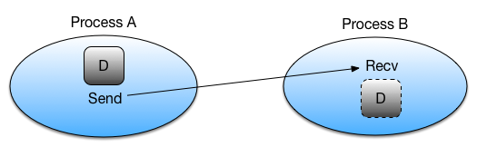
To get an idea of how communication typically happens, imagine we have two ranks: rank A and rank B. If rank A wants to send data to rank B (e.g., point-to-point), it must first call the appropriate MPI send function which typically (but not always, as we’ll find out later) puts that data into an internal buffer; known as the send buffer or the envelope. Once the data is in the buffer, MPI figures out how to route the message to rank B (usually over a network) and then sends it to B. To receive the data, rank B must call a data receiving function which will listen for messages being sent to it. In some cases, rank B will then send an acknowledgement to say that the transfer has finished, similar to read receipts in e-mails and instant messages.
Check your understanding
Consider a simulation where each rank calculates the physical properties for a subset of cells on a very large grid of points. One step of the calculation needs to know the average temperature across the entire grid of points. How would you approach calculating the average temperature?
Solution
There are multiple ways to approach this situation, but the most efficient approach would be to use collective operations to send the average temperature to a main rank which performs the final calculation. You can, of course, also use a point-to-point pattern, but it would be less efficient, especially with a large number of ranks.
If the simulation wasn’t done in parallel, or was instead using shared-memory parallelism, such as OpenMP, we wouldn’t need to do any communication to get the data required to calculate the average.
MPI data types
When we send a message, MPI needs to know the size of the data being transferred. The size is not the number of bytes of data being sent, as you may expect, but is instead the number of elements of a specific data type being sent. When we send a message, we have to tell MPI how many elements of “something” we are sending and what type of data it is. If we don’t do this correctly, we’ll either end up telling MPI to send only some of the data or try to send more data than we want! For example, if we were sending an array and we specify too few elements, then only a subset of the array will be sent or received. But if we specify too many elements, than we are likely to end up with either a segmentation fault or undefined behaviour! And the same can happen if we don’t specify the correct data type.
There are two types of data type in MPI: “basic” data types and derived data types. The basic data types are in essence
the same data types we would use in C such as int, float, char and so on. However, MPI doesn’t use the same
primitive C types in its API, using instead a set of constants which internally represent the data types. These data
types are in the table below:
| MPI basic data type | C equivalent |
|---|---|
| MPI_SHORT | short int |
| MPI_INT | int |
| MPI_LONG | long int |
| MPI_LONG_LONG | long long int |
| MPI_UNSIGNED_CHAR | unsigned char |
| MPI_UNSIGNED_SHORT | unsigned short int |
| MPI_UNSIGNED | unsigned int |
| MPI_UNSIGNED_LONG | unsigned long int |
| MPI_UNSIGNED_LONG_LONG | unsigned long long int |
| MPI_FLOAT | float |
| MPI_DOUBLE | double |
| MPI_LONG_DOUBLE | long double |
| MPI_BYTE | char |
Remember, these constants aren’t the same as the primitive types in C, so we can’t use them to create variables, e.g.,
MPI_INT my_int = 1;
is not valid code because, under the hood, these constants are actually special data structures used by MPI. Therefore we can only them as arguments in MPI functions.
Don’t forget to update your types
At some point during development, you might change an
intto alongor afloatto adouble, or something to something else. Once you’ve gone through your codebase and updated the types for, e.g., variable declarations and function arguments, you must do the same for MPI functions. If you don’t, you’ll end up running into communication errors. It could be helpful to define compile-time constants for the data types and use those instead. If you ever do need to change the type, you would only have to do it in one place, e.g.:// define constants for your data types #define MPI_INT_TYPE MPI_INT #define INT_TYPE int // use them as you would normally INT_TYPE my_int = 1;
Derived data types, on the other hand, are very similar to C structures which we define by using the basic MPI data types. They’re often useful to group together similar data in communications, or when you need to send a structure from one rank to another. This will be covered in more detail in the Advanced Communication Techniques episode.
What type should you use?
For the following pieces of data, what MPI data types should you use?
a[] = {1, 2, 3, 4, 5};a[] = {1.0, -2.5, 3.1456, 4591.223, 1e-10};a[] = "Hello, world!";Solution
The fact that
a[]is an array does not matter, because all of the elemnts ina[]will be the same data type. In MPI, as we’ll see in the next episode, we can either send a single value or multiple values (in an array).
MPI_INTMPI_DOUBLE-MPI_FLOATwould not be correct asfloat’s contain 32 bits of data whereasdouble’s are 64 bit.MPI_BYTEorMPI_CHAR- you may want to use strlen to calculate how many elements ofMPI_CHARbeing sent
Communicators
All communication in MPI is handled by something known as a communicator. We can think of a communicator as being a
collection of ranks which are able to exchange data with one another. What this means is that every communication
between two (or more) ranks is linked to a specific communicator. When we run an MPI application, every rank will belong
to the default communicator known as MPI_COMM_WORLD. We’ve seen this in earlier episodes when, for example, we’ve used
functions like MPI_Comm_rank() to get the rank number,
int my_rank;
MPI_Comm_rank(MPI_COMM_WORLD, &my_rank);  // MPI_COMM_WORLD is the communicator the rank belongs to
In addition to MPI_COMM_WORLD, we can make sub-communicators and distribute ranks into them. Messages can only be sent
and received to and from the same communicator, effectively isolating messages to a communicator. For most applications,
we usually don’t need anything other than MPI_COMM_WORLD. But organising ranks into communicators can be helpful in
some circumstances, as you can create small “work units” of multiple ranks to dynamically schedule the workload, create
one communicator for each physical hardware node on a HPC cluster, or to help compartmentalise the problem into smaller
chunks by using a virtual cartesian topology.
Throughout this course, we will stick to using MPI_COMM_WORLD.
Communication modes
When sending data between ranks, MPI will use one of four communication modes: synchronous, buffered, ready or standard. When a communication function is called, it takes control of program execution until the send-buffer is safe to be re-used again. What this means is that it’s safe to re-use the memory/variable you passed without affecting the data that is still being sent. If MPI didn’t have this concept of safety, then you could quite easily overwrite or destroy any data before it is transferred fully! This would lead to some very strange behaviour which would be hard to debug. The difference between the communication mode is when the buffer becomes safe to re-use. MPI won’t guess at which mode should be used. That is up to the programmer. Therefore each mode has an associated communication function:
| Mode | Blocking function |
|---|---|
| Synchronous | MPI_SSend() |
| Buffered | MPI_Bsend() |
| Ready | MPI_Rsend() |
| Standard | MPI_Send() |
In contrast to the four modes for sending data, receiving data only has one mode and therefore only a single function.
| Mode | MPI Function |
|---|---|
| Standard | MPI_Recv() |
Synchronous sends
In synchronous communication, control is returned when the receiving rank has received the data and sent back, or “posted”, confirmation that the data has been received. It’s like making a phone call. Data isn’t exchanged until you and the person have both picked up the phone, had your conversation and hung the phone up.
Synchronous communication is typically used when you need to guarantee synchronisation, such as in iterative methods or time dependent simulations where it is vital to ensure consistency. It’s also the easiest communication mode to develop and debug with because of its predictable behaviour.
Buffered sends
In a buffered send, the data is written to an internal buffer before it is sent and returns control back as soon as the
data is copied. This means MPI_Bsend() returns before the data has been received by the receiving rank, making this an
asynchronous type of communication as the sending rank can move onto its next task whilst the data is transmitted. This
is just like sending a letter or an e-mail to someone. You write your message, put it in an envelope and drop it off in
the postbox. You are blocked from doing other tasks whilst you write and send the letter, but as soon as it’s in the
postbox, you carry on with other tasks and don’t wait for the letter to be delivered!
Buffered sends are good for large messages and for improving the performance of your communication patterns by taking advantage of the asynchronous nature of the data transfer.
Ready sends
Ready sends are different to synchronous and buffered sends in that they need a rank to already be listening to receive a message, whereas the other two modes can send their data before a rank is ready. It’s a specialised type of communication used only when you can guarantee that a rank will be ready to receive data. If this is not the case, the outcome is undefined and will likely result in errors being introduced into your program. The main advantage of this mode is that you eliminate the overhead of having to check that the data is ready to be sent, and so is often used in performance critical situations.
You can imagine a ready send as like talking to someone in the same room, who you think is listening. If they are listening, then the data is transferred. If it turns out they’re absorbed in something else and not listening to you, then you may have to repeat yourself to make sure your transmit the information you wanted to!
Standard sends
The standard send mode is the most commonly used type of send, as it provides a balance between ease of use and performance. Under the hood, the standard send is either a buffered or a synchronous send, depending on the availability of system resources (e.g. the size of the internal buffer) and which mode MPI has determined to be the most efficient.
Which mode should I use?
Each communication mode has its own use cases where it excels. However, it is often easiest, at first, to use the standard send,
MPI_Send(), and optimise later. If the standard send doesn’t meet your requirements, or if you need more control over communication, then pick which communication mode suits your requirements best. You’ll probably need to experiment to find the best!
Communication mode summary
Mode Description Analogy MPI Function Synchronous Returns control to the program when the message has been sent and received successfully. Making a phone call MPI_Ssend()Buffered Returns control immediately after copying the message to a buffer, regardless of whether the receive has happened or not. Sending a letter or e-mail MPI_Bsend()Ready Returns control immediately, assuming the matching receive has already been posted. Can lead to errors if the receive is not ready. Talking to someone you think/hope is listening MPI_Rsend()Standard Returns control when it’s safe to reuse the send buffer. May or may not wait for the matching receive (synchronous mode), depending on MPI implementation and message size. Phone call or letter MPI_Send()
Blocking and non-blocking communication
In addition to the communication modes, communication is done in two ways: either by blocking execution until the communication is complete (like how a synchronous send blocks until an receive acknowledgment is sent back), or by returning immediately before any part of the communication has finished, with non-blocking communication. Just like with the different communication modes, MPI doesn’t decide if it should use blocking or non-blocking communication calls. That is, again, up to the programmer to decide. As we’ll see in later episodes, there are different functions for blocking and non-blocking communication.
A blocking synchronous send is one where the message has to be sent from rank A, received by B and an acknowledgment sent back to A before the communication is complete and the function returns. In the non-blocking version, the function returns immediately even before rank A has sent the message or rank B has received it. It is still synchronous, so rank B still has to tell A that it has received the data. But, all of this happens in the background so other work can continue in the foreground which data is transferred. It is then up to the programmer to check periodically if the communication is done – and to not modify/use the data/variable/memory before the communication has been completed.
Is
MPI_Bsend()non-blocking?The buffered communication mode is a type of asynchronous communication, because the function returns before the data has been received by another rank. But, it’s not a non-blocking call unless you use the non-blocking version
MPI_Ibsend()(more on this later). Even though the data transfer happens in the background, allocating and copying data to the send buffer happens in the foreground, blocking execution of our program. On the other hand,MPI_Ibsend()is “fully” asynchronous because even allocating and copying data to the send buffer happens in the background.
One downside to blocking communication is that if rank B is never listening for messages, rank A will become deadlocked. A deadlock happens when your program hangs indefinitely because the send (or receive) is unable to complete. Deadlocks occur for a countless number of reasons. For example, we may forget to write the corresponding receive function when sending data. Or a function may return earlier due to an error which isn’t handled properly, or a while condition may never be met creating an infinite loop. Ranks can also can silently, making communication with them impossible, but this doesn’t stop any attempts to send data to crashed rank.
Avoiding communication deadlocks
A common piece of advice in C is that when allocating memory using
malloc(), always write the accompanying call tofree()to help avoid memory leaks by forgetting to deallocate the memory later. You can apply the same mantra to communication in MPI. When you send data, always write the code to receive the data as you may forget to later and accidentally cause a deadlock.
Blocking communication works best when the work is balanced across ranks, so that each rank has an equal amount of things to do. A common pattern in scientific computing is to split a calculation across a grid and then to share the results between all ranks before moving onto the next calculation. If the workload is well balanced, each rank will finish at roughly the same time and be ready to transfer data at the same time. But, as shown in the diagram below, if the workload is unbalanced, some ranks will finish their calculations earlier and begin to send their data to the other ranks before they are ready to receive data. This means some ranks will be sitting around doing nothing whilst they wait for the other ranks to become ready to receive data, wasting computation time.

If most of the ranks are waiting around, or one rank is very heavily loaded in comparison, this could massively impact the performance of your program. Instead of doing calculations, a rank will be waiting for other ranks to complete their work.
Non-blocking communication hands back control, immediately, before the communication has finished. Instead of your program being blocked by communication, ranks will immediately go back to the heavy work and instead periodically check if there is data to receive (which is up to the programmer) instead of waiting around. The advantage of this communication pattern is illustrated in the diagram below, where less time is spent communicating.
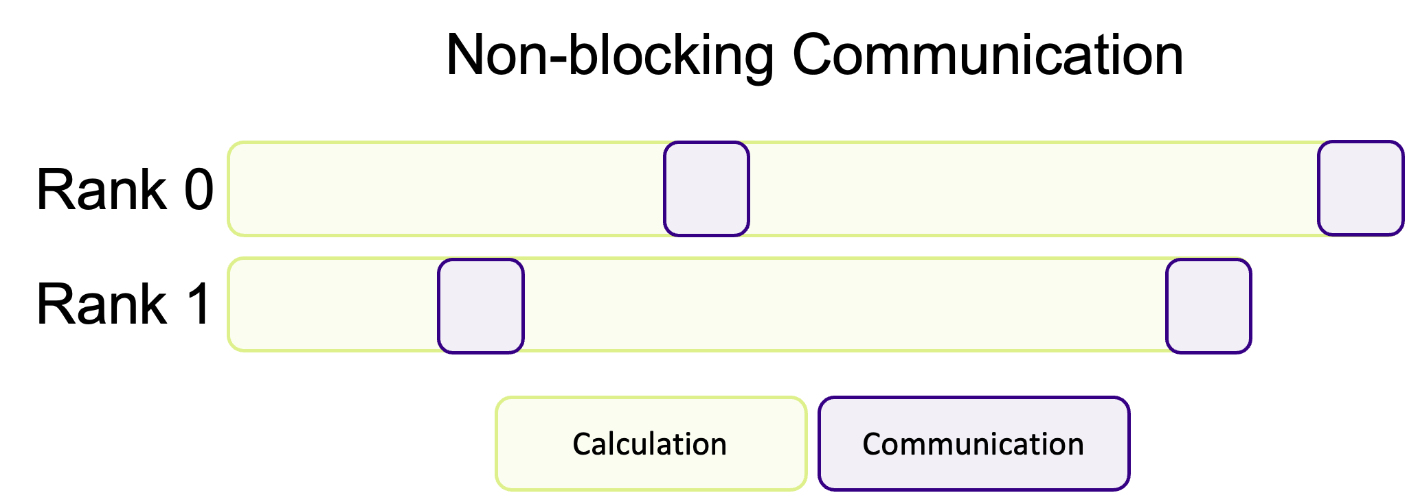
This is a common pattern where communication and calculations are interwoven with one another, decreasing the amount of “dead time” where ranks are waiting for other ranks to communicate data. Unfortunately, non-blocking communication is often more difficult to successfully implement and isn’t appropriate for every algorithm. In most cases, blocking communication is usually easier to implement and to conceptually understand, and is somewhat “safer” in the sense that the program cannot continue if data is missing. However, the potential performance improvements of overlapping communication and calculation is often worth the more difficult implementation and harder to read/more complex code.
Should I use blocking or non-blocking communication?
When you are first implementing communication into your program, it’s advisable to first use blocking synchronous sends to start with, as this is arguably the easiest to use pattern. Once you are happy that the correct data is being communicated successfully, but you are unhappy with performance, then it would be time to start experimenting with the different communication modes and blocking vs. non-blocking patterns to balance performance with ease of use and code readability and maintainability.
MPI communication in everyday life?
We communicate with people non-stop in everyday life, whether we want to or not! Think of some examples/analogies of blocking and non-blocking communication we use to talk to other people.
Solution
Probably the most common example of blocking communication in everyday life would be having a conversation or a phone call with someone. The conversation can’t happen and data can’t be communicated until the other person responds or picks up the phone. Until the other person responds, we are stuck waiting for the response.
Sending e-mails or letters in the post is a form of non-blocking communication we’re all familiar with. When we send an e-mail, or a letter, we don’t wait around to hear back for a response. We instead go back to our lives and start doing tasks instead. We can periodically check our e-mail for the response, and either keep doing other tasks or continue our previous task once we’ve received a response back from our e-mail.
Key Points
Data is sent between ranks using “messages”
Messages can either block the program or be sent/received asynchronously
Knowing the exact amount of data you are sending is required
Point-to-Point Communication
Overview
Teaching: 10 min
Exercises: 10 minQuestions
How do I send data between processes?
Objectives
Describe what is meant by point-to-point communication
Describe the arguments to MPI_Send() and MPI_Recv()
Use MPI_Send() to send a message to another rank
Use MPI_Recv() to receive a message from another rank
Write, compile and run a complete program that sends a message from one rank to another
In the previous episode we introduced the various types of communication in MPI.
In this section we will use the MPI library functions MPI_Send() and
MPI_Recv(), which employ point-to-point communication, to send data from one rank to another.
Let’s look at how MPI_Send() and MPI_Recv()are typically used:
- Rank A decides to send data to rank B. It first packs the data to send into a buffer, from which it will be taken.
- Rank A then calls
MPI_Send()to create a message for rank B. The underlying MPI communication is then given the responsibility of routing the message to the correct destination. - Rank B must know that it is about to receive a message and acknowledge this
by calling
MPI_Recv(). This sets up a buffer for writing the incoming data when it arrives and instructs the communication device to listen for the message.
As mentioned in the previous episode, MPI_Send() and MPI_Recv() are synchronous operations,
and will not return until the communication on both sides is complete.
Sending a Message: MPI_Send
The MPI_Send() function is defined as follows:
int MPI_Send(
    void *data,
    int count,
    MPI_Datatype datatype,
    int destination,
    int tag,
    MPI_Comm communicator)
data: |
Pointer to the start of the data being sent. We would not expect this to change, hence it’s defined as const |
count: |
Number of elements to send |
datatype: |
The type of the element data being sent, e.g. MPI_INTEGER, MPI_CHAR, MPI_FLOAT, MPI_DOUBLE, … |
destination: |
The rank number of the rank the data will be sent to |
tag: |
An message tag (integer), which is used to differentiate types of messages. We can specify 0 if we don’t need different types of messages |
communicator: |
The communicator, e.g. MPI_COMM_WORLD as seen in previous episodes |
For example, if we wanted to send a message that contains "Hello, world!\n" from rank 0 to rank 1, we could state
(assuming we were rank 0):
char *message = "Hello, world!\n";
MPI_Send(message, 14, MPI_CHAR, 1, 0, MPI_COMM_WORLD);
So we are sending 14 elements of MPI_CHAR one time, and specified 0 for our message tag since we don’t anticipate
having to send more than one type of message. This call is synchronous, and will block until the corresponding
MPI_Recv() operation receives and acknowledges receipt of the message.
MPI_Ssend: an Alternative to MPI_Send
MPI_Send()represents the “standard mode” of sending messages to other ranks, but some aspects of its behaviour are dependent on both the implementation of MPI being used, and the circumstances of its use: there are three scenarios to consider:
- The message is directly passed to the receive buffer, in which case the communication has completed
- The send message is buffered within some internal MPI buffer but hasn’t yet been received
- The function call waits for a corresponding receiving process
In scenarios 1 & 2, the call is able to return immediately, but with 3 it may block until the recipient is ready to receive. It is dependent on the MPI implementation as to what scenario is selected, based on performance, memory, and other considerations.
A very similar alternative to
MPI_Send()is to useMPI_Ssend()- synchronous send - which ensures the communication is both synchronous and blocking. This function guarantees that when it returns, the destination has categorically started receiving the message.
Receiving a Message: MPI_Recv
Conversely, the MPI_Recv() function looks like the following:
int MPI_Recv(
    void *data,
    int count,
    MPI_Datatype datatype,
    int source,
    int tag,
    MPI_Comm communicator,
    MPI_Status *status)
data: |
Pointer to where the received data should be written |
count: |
Maximum number of elements to receive |
datatype: |
The type of the data being received |
source: |
The number of the rank sending the data |
tag: |
A message tag (integer), which must either match the tag in the sent message, or if MPI_ANY_TAG is specified, a message with any tag will be accepted |
communicator: |
The communicator (we have used MPI_COMM_WORLD in earlier examples) |
status: |
A pointer for writing the exit status of the MPI command, indicating whether the operation succeeded or failed |
Continuing our example, to receive our message we could write:
char message[15];
MPI_Status status;
MPI_Recv(message, 14, MPI_CHAR, 0, 0, MPI_COMM_WORLD, &status);
Here, we create our buffer to receive the data, as well as a variable to hold the exit status of the receive operation.
We then call MPI_Recv(), specifying our returned data buffer, the number of elements we will receive (14) which will be
of type MPI_CHAR and sent by rank 0, with a message tag of 0.
As with MPI_Send(), this call will block - in this case until the message is received and acknowledgement is sent
to rank 0, at which case both ranks will proceed.
Let’s put this together with what we’ve learned so far.
Here’s an example program that uses MPI_Send() and MPI_Recv() to send the string "Hello World!"
from rank 0 to rank 1:
#include <stdio.h>
#include <mpi.h>

int main(int argc, char **argv) {
  int rank, n_ranks;

  // First call MPI_Init
  MPI_Init(&argc, &argv);

  // Check that there are two ranks
  MPI_Comm_size(MPI_COMM_WORLD, &n_ranks);
  if (n_ranks != 2) {
    printf("This example requires exactly two ranks\n");
    MPI_Finalize();
    return 1;
  }

  // Get my rank
  MPI_Comm_rank(MPI_COMM_WORLD,&rank);

  if (rank == 0) {
     char *message = "Hello, world!\n";
     MPI_Send(message, 14, MPI_CHAR, 1, 0, MPI_COMM_WORLD);
  }

  if (rank == 1) {
     char message[14];
     MPI_Status status;
     MPI_Recv(message, 14, MPI_CHAR, 0, 0, MPI_COMM_WORLD, &status);
     printf("%s",message);
  }

  // Call finalize at the end
  return MPI_Finalize();
}
MPI Data Types in C
In the above example we send a string of characters and therefore specify the type
MPI_CHAR. For a complete list of types, see the MPICH documentation.
Try It Out
Compile and run the above code. Does it behave as you expect?
Solution
mpicc mpi_hello_world.c -o mpi_hello_world
mpirun -n 2 mpi_hello_world
Note above that we specified only 2 ranks, since that’s what the program requires (see line 12). You should see:
Hello, world!
What Happens If…
Try modifying, compiling, and re-running the code to see what happens if you…
- Change the tag integer of the sent message. How could you resolve this where the message is received?
- Modify the element count of the received message to be smaller than that of the sent message. How could you resolve this in how the message is sent?
Solution
- The program will hang since it’s waiting for a message with a tag that will never be sent (press
Ctrl-Cto kill the hanging process). To resolve this, make the tag inMPI_Recv()match the tag you specified inMPI_Send().- You will likely see a message like the following:
[...:220695] *** An error occurred in MPI_Recv
[...:220695] *** reported by process [2456485889,1]
[...:220695] *** on communicator MPI_COMM_WORLD
[...:220695] *** MPI_ERR_TRUNCATE: message truncated
[...:220695] *** MPI_ERRORS_ARE_FATAL (processes in this communicator will now abort,
[...:220695] ***    and potentially your MPI job)
You could resolve this by sending a message of equal size, truncating the message. A related question is whether this fix makes any sense!
Many Ranks
Change the above example so that it works with any number of ranks. Pair even ranks with odd ranks and have each even rank send a message to the corresponding odd rank.
Solution
#include <stdio.h>
#include <mpi.h>

int main(int argc, char **argv) {
    int rank, n_ranks, my_pair;

    // First call MPI_Init
    MPI_Init(&argc, &argv);

    // Get the number of ranks
    MPI_Comm_size(MPI_COMM_WORLD,&n_ranks);

    // Get my rank
    MPI_Comm_rank(MPI_COMM_WORLD,&rank);

    // Figure out my pair
    if (rank % 2 == 1) {
       my_pair = rank - 1;
    } else {
       my_pair = rank + 1;
    }

    // Run only if my pair exists
    if (my_pair < n_ranks) {
       if (rank % 2 == 0) {
           char *message = "Hello, world!\n";
           MPI_Send(message, 14, MPI_CHAR, my_pair, 0, MPI_COMM_WORLD);
       }

       if (rank % 2 == 1) {
           char message[14];
           MPI_Status  status;
           MPI_Recv(message, 14, MPI_CHAR, my_pair, 0, MPI_COMM_WORLD, &status);
           printf("%s",message);
        }
    }

    // Call finalize at the end
    return MPI_Finalize();
}
Hello Again, World!
Modify the Hello World code below so that each rank sends its message to rank 0. Have rank 0 print each message.
#include <stdio.h>
#include <mpi.h>

int main(int argc, char **argv) {
    int rank;
    int message[30];

    // First call MPI_Init
    MPI_Init(&argc, &argv);

    // Get my rank
    MPI_Comm_rank(MPI_COMM_WORLD, &rank);

    // Print a message using snprintf and then printf
    snprintf(message, 30, "Hello World, I'm rank %d", rank);
    printf("%s\n", message);

    // Call finalize at the end
    return MPI_Finalize();
}
Solution
#include <stdio.h>
#include <mpi.h>

int main(int argc, char **argv) {
    int rank, n_ranks, numbers_per_rank;

    // First call MPI_Init
    MPI_Init(&argc, &argv);
    // Get my rank and the number of ranks
    MPI_Comm_rank(MPI_COMM_WORLD, &rank);
    MPI_Comm_size(MPI_COMM_WORLD, &n_ranks);

    if (rank != 0) {
       // All ranks other than 0 should send a message

       char message[30];
       sprintf(message, "Hello World, I'm rank %d\n", rank);
       MPI_Send(message, 30, MPI_CHAR, 0, 0, MPI_COMM_WORLD);

    } else {
       // Rank 0 will receive each message and print them

       for( int sender = 1; sender < n_ranks; sender++ ) {
          char message[30];
          MPI_Status status;

          MPI_Recv(message, 30, MPI_CHAR, sender, 0, MPI_COMM_WORLD, &status);
          printf("%s",message);
       }
    }

    // Call finalize at the end
    return MPI_Finalize();
}
Blocking
Try the code below with two ranks and see what happens. How would you change the code to fix the problem?
Note: If you are using MPICH, this example might work. With OpenMPI it shouldn’t!
#include <mpi.h>

#define ARRAY_SIZE 3

int main(int argc, char **argv) {
    MPI_Init(&argc, &argv);

    int rank;
    MPI_Comm_rank(MPI_COMM_WORLD, &rank);

    const int comm_tag = 1;
    int numbers[ARRAY_SIZE] = {1, 2, 3};
    MPI_Status recv_status;

    if (rank == 0) {
        // synchronous send: returns when the destination has started to
        // receive the message
        MPI_Ssend(&numbers, ARRAY_SIZE, MPI_INT, 1, comm_tag, MPI_COMM_WORLD);
        MPI_Recv(&numbers, ARRAY_SIZE, MPI_INT, 1, comm_tag, MPI_COMM_WORLD, &recv_status);
    } else {
        MPI_Ssend(&numbers, ARRAY_SIZE, MPI_INT, 0, comm_tag, MPI_COMM_WORLD);
        MPI_Recv(&numbers, ARRAY_SIZE, MPI_INT, 0, comm_tag, MPI_COMM_WORLD, &recv_status);
    }

    return MPI_Finalize();
}
Solution
MPI_Send()will block execution until the receiving process has calledMPI_Recv(). This prevents the sender from unintentionally modifying the message buffer before the message is actually sent. Above, both ranks callMPI_Send()and just wait for the other to respond. The solution is to have one of the ranks receive its message before sending.Sometimes
MPI_Send()will actually make a copy of the buffer and return immediately. This generally happens only for short messages. Even when this happens, the actual transfer will not start before the receive is posted.For this example, let’s have rank 0 send first, and rank 1 receive first. So all we need to do to fix this is to swap the send and receive for rank 1:
if (rank == 0) {
   MPI_Ssend(&numbers, ARRAY_SIZE, MPI_INT, 1, comm_tag, MPI_COMM_WORLD);
   MPI_Recv(&numbers, ARRAY_SIZE, MPI_INT, 1, comm_tag, MPI_COMM_WORLD, &recv_status);
} else {
   // Change the order, receive then send
   MPI_Recv(&numbers, ARRAY_SIZE, MPI_INT, 0, comm_tag, MPI_COMM_WORLD, &recv_status);
   MPI_Ssend(&numbers, ARRAY_SIZE, MPI_INT, 0, comm_tag, MPI_COMM_WORLD);
}
Ping Pong
Write a simplified simulation of Ping Pong according to the following rules:
- Ranks 0 and 1 participate
- Rank 0 starts with the ball
- The rank with the ball sends it to the other rank
- Both ranks count the number of times they get the ball
- After counting to 1 million, the rank is bored and gives up
- There are no misses or points
Solution
#include <stdio.h>
#include <mpi.h>

int main(int argc, char **argv) {
    int rank, neighbour;
    int max_count = 1000000;
    int counter;
    int bored;
    int ball = 1; // A dummy message to simulate the ball
    MPI_Status status;

    // First call MPI_Init
    MPI_Init(&argc, &argv);

    // Get my rank
    MPI_Comm_rank(MPI_COMM_WORLD, &rank);

    // Call the other rank the neighbour
    if (rank == 0) {
        neighbour = 1;
    } else {
        neighbour = 0;
    }

    if (rank == 0) {
        // Rank 0 starts with the ball. Send it to rank 1
        MPI_Send(&ball, 1, MPI_INT, 1, 0, MPI_COMM_WORLD);
    }

    // Now run a send and receive in a loop until someone gets bored
    // the behaviour is the same for both ranks
    counter = 0;
    bored = 0;
    while (!bored) {
        // Receive the ball
        MPI_Recv(&ball, 1, MPI_INT, neighbour, 0, MPI_COMM_WORLD, &status);

        // Increment the counter and send the ball back
        counter += 1;
        MPI_Send(&ball, 1, MPI_INT, neighbour, 0, MPI_COMM_WORLD);

        // Check if the rank is bored
        bored = counter >= max_count;
    }
    printf("rank %d is bored and giving up \n", rank);

    // Call finalize at the end
    return MPI_Finalize();
}
Key Points
Use
MPI_Send()andMPI_Recv()to send and receive data between ranksUsing
MPI_Ssend()will always block the sending rank until the message is receivedUsing
MPI_Send()may block the sending rank until the message is received, depending on whether the message is buffered and the buffer is available for reuseUsing
MPI_Recv()will always block the receiving rank until the message is received
Collective Communication
Overview
Teaching: 0 min
Exercises: 0 minQuestions
How do I get data to more than one rank?
Objectives
Describe what is meant by collective communication, and its advantages
Describe how to synchronise ranks using MPI
Broadcast a message to multiple ranks
Describe how to split and send data across multiple ranks, and receive data from multiple ranks
Describe how to “reduce” values from across multiple ranks
Describe how to perform broadcasting and reduction in a single MPI call
The previous episode showed how to send data from one rank to another using point-to-point communication. If we wanted to send data from multiple ranks to a single rank to, for example, add up the value of a variable across multiple ranks, we have to manually loop over each rank to communicate the data. This type of communication, where multiple ranks talk to one another known as called collective communication. In the code example below, point-to-point communication is used to calculate the sum of the rank numbers - feel free to try it out!
#include <stdio.h>
#include <mpi.h>

int main(int argc, char **argv) {
    int my_rank, num_ranks;

    // First call MPI_Init
    MPI_Init(&argc, &argv);

    MPI_Comm_rank(MPI_COMM_WORLD, &my_rank);
    MPI_Comm_size(MPI_COMM_WORLD, &num_ranks);

    int sum;
    MPI_Status status;

    // Rank 0 is the "root" rank, where we'll receive data and sum it up
    if (my_rank == 0) {
        sum = my_rank;

        // Start by receiving the rank number from every rank, other than itself
        for (int i = 1; i < num_ranks; ++i) {
            int recv_num;
            MPI_Recv(&recv_num, 1, MPI_INT, i, 0, MPI_COMM_WORLD, &status);
            sum += recv_num;
        }
        // Now sum has been calculated, send it back to every rank other than the root
        for (int i = 1; i < num_ranks; ++i) {
            MPI_Send(&sum, 1, MPI_INT, i, 0, MPI_COMM_WORLD);
        }
    } else {  // All other ranks will send their rank number and receive sum */
        MPI_Send(&my_rank, 1, MPI_INT, 0, 0, MPI_COMM_WORLD);
        MPI_Recv(&sum, 1, MPI_INT, 0, 0, MPI_COMM_WORLD, &status);
    }

    printf("Rank %d has a sum of %d\n", my_rank, sum);

    // Call finalize at the end
    return MPI_Finalize();
}
For it’s use case, the code above works perfectly fine. However, it isn’t very efficient when you need to communicate large amounts of data, have lots of ranks, or when the workload is uneven (due to the blocking communication). It’s also a lot of code to not do very much, which makes it easy to introduce mistakes in our code. Another mistake in this example
would be to start the loop over ranks from 0, which would cause a deadlock! It’s actually quite a common mistake for new MPI users to write something like the above.
We don’t need to write code like this (unless we want complete control over the data communication), because MPI has access to collective communication functions to abstract all of this code for us. The above code can be replaced by a single collective communication function. Collection operations are also implemented far more efficiently in the MPI library than we could ever write using point-to-point communications.
There are several collective operations that are implemented in the MPI standard. The most commonly-used are:
| Type | Description |
|---|---|
| Synchronisation | Wait until all processes have reached the same point in the program. |
| One-To-All | One rank sends the same message to all other ranks. |
| All-to-One | All ranks send data to a single rank. |
| All-to-All | All ranks have data and all ranks receive data. |
Synchronisation
Barrier
The most simple form of collective communication is a barrier. Barriers are used to synchronise ranks by adding a point
in a program where ranks must wait until all ranks have reached the same point. A barrier is a collective operation
because all ranks need to communicate with one another to know when they can leave the barrier. To create a barrier, we
use the MPI_Barrier() function,
int MPI_Barrier(
    MPI_Comm comm
);
comm: |
The communicator to add a barrier to |
When a rank reaches a barrier, it will pause and wait for all the other ranks to catch up and reach the barrier as well. As ranks waiting at a barrier aren’t doing anything, barriers should be used sparingly to avoid large synchronisation overheads, which affects the scalability of our program. We should also avoid using barriers in parts of our program has have complicated branches, as we may introduce a deadlock by having a barrier in only one branch.
In practise, there are not that many practical use cases for a barrier in an MPI application. In a shared-memory environment, synchronisation is important to ensure consistent and controlled access to shared data. But in MPI, where each rank has its own private memory space and often resources, it’s rare that we need to care about ranks becoming out-of-sync. However, one usecase is when multiple ranks need to write sequentially to the same file. The code example below shows how you may handle this by using a barrier.
for (int i = 0; i < num_ranks; ++i) {
    if (i == my_rank) {           /* One rank writes to the file */
        write_to_file();
    }
    MPI_Barrier(MPI_COMM_WORLD);  /* Wait for data to be written, so it is sequential and ordered */
}
One-To-All
Broadcast
We’ll often find that we need to data from one rank to all the other ranks. One approach, which is not very efficient,
is to use MPI_Send() in a loop to send the data from rank to rank one by one. A far more efficient approach is to use
the collective function MPI_Bcast() to broadcast the data from a root rank to every other rank. The MPI_Bcast()
function has the following arguments,
int MPI_Bcast(
    void *data,
    int count,
    MPI_Datatype datatype,
    int root,
    MPI_Comm comm
);
data: |
The data to be sent to all ranks |
count: |
The number of elements of data |
datatype: |
The datatype of the data |
root: |
The rank which data will be sent from |
comm: |
The communicator containing the ranks to broadcast to |
MPI_Bcast() is similar to the MPI_Send() function, but MPI_Bcast() sends
the data to all ranks (other than itself, where the data already is) instead of a single rank, as shown in the
diagram below.
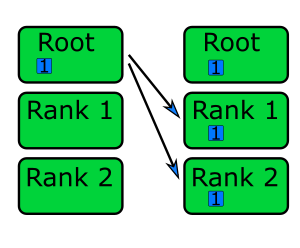
There are lots of use cases for broadcasting data. One common case is when data is sent back to a “root” rank to process, which then broadcasts the results back out to all the other ranks. Another example, shown in the code exert below, is to read data in on the root rank and to broadcast it out. This is useful pattern on some systems where there are not enough resources (filesystem bandwidth, limited concurrent I/O operations) for every ranks to read the file at once.
int data_from_file[NUM_POINTS]

/* Read in data from file, and put it into data_from_file. We are only reading data
   from the root rank (rank 0), as multiple ranks reading from the same file at the
   same time can sometimes result in problems or be slower */
if (my_rank == 0) {
    get_data_from_file(data_from_file);
}

/* Use MPI_Bcast to send the data to every other rank */
MPI_Bcast(data_from_file, NUM_POINTS, MPI_INT, 0, MPI_COMM_WORLD);
Sending greetings
Send a message from rank 0 saying “Hello from rank 0” to all ranks using
MPI_Bcast().Solution
#include <mpi.h>
#include <stdio.h>
#include <string.h>

#define NUM_CHARS 32

int main(int argc, char **argv) {
    int my_rank, num_ranks;
    MPI_Init(&argc, &argv);
    MPI_Comm_rank(MPI_COMM_WORLD, &my_rank);
    MPI_Comm_size(MPI_COMM_WORLD, &num_ranks);

    char message[NUM_CHARS];

    if (my_rank == 0) {
        strcpy(message, "Hello from rank 0");
    }

    MPI_Bcast(message, NUM_CHARS, MPI_CHAR, 0, MPI_COMM_WORLD);
    printf("I'm rank %d and I got the message '%s'\n", my_rank, message);

    return MPI_Finalize();
}
Scatter
One way to parallelise processing amount of data is to have ranks process a subset of the data. One method for
distributing the data to each rank is to have a root rank which prepares the data, and then send the data to every rank.
The communication could be done manually using point-to-point communication, but it’s easier, and faster, to use a
single collective communication. We can use MPI_Scatter() to split the data into equal sized chunks and communicate
a diferent chunk to each rank, as shown in the diagram below.
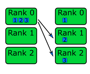
MPI_Scatter() has the following arguments,
int MPI_Scatter(
    void *sendbuf,
    int sendcount,
    MPI_Datatype sendtype,
    void *recvbuffer,
    int recvcount,
    MPI_Datatype recvtype,
    int root,
    MPI_Comm comm
);
*sendbuf: |
The data to be scattered across ranks (only important for the root rank) |
sendcount: |
The number of elements of data to send to each root rank (only important for the root rank) |
sendtype: |
The data type of the data being sent (only important for the root rank) |
*recvbuffer: |
A buffer to receive data into, including the root rank |
recvcount: |
Th number of elements of data to receive. Usually the same as sendcount |
recvtype: |
The data type of the data being received. Usually the same as sendtype |
root: |
The rank data is being scattered from |
comm: |
The communicator |
The data to be scattered is split into even chunks of size sendcount. If sendcount is 2 and sendtype is
MPI_INT, then each rank will receive two integers. The values for recvcount and recvtype are the same as
sendcount and sendtype. If the total amount of data is not evenly divisible by the number of processes,
MPI_Scatter() will not work. In this case, we need to use
MPI_Scatterv() instead to specify the amount of data each
rank will receive. The code example below shows MPI_Scatter() being used to send data which has been initialised only
on the root rank.
#define ROOT_RANK 0

int send_data[NUM_DATA_POINTS]

if (my_rank == ROOT_RANK) {
    initialise_send_data(send_data);  /* The data which we're going to scatter only needs to exist in the root rank */
}

/* Calculate the elements of data each rank will get, and allocate space for
   the receive buffer -- we are assuming NUM_DATA_POINTS is divisible by num_ranks */
int num_per_rank = NUM_DATA_POINTS / num_ranks;
int *scattered_data_for_rank = malloc(num_per_rank * sizeof(int));


/* Using a single function call, the data has been split and communicated evenly between all ranks */
MPI_Scatter(send_data, num_per_rank, MPI_INT, scattered_data_for_rank, num_per_rank, MPI_INT, ROOT_RANK, MPI_COMM_WORLD);
All-To-One
Gather
The opposite of scattering from one rank to multiple, is to gather data from multiple ranks into a single rank. We can
do this by using the collection function MPI_Gather(), which has the arguments,
int MPI_Gather(
    void *sendbuf,
    int sendcount,
    MPI_Datatype sendtype,
    void *recvbuff,
    int recvcount,
    MPI_Datatype recvtype,
    int root,
    MPI_Comm comm
);
*sendbuff: |
The data to send to the root rank |
sendcount: |
The number of elements of data to send |
sendtype: |
The data type of the data being sent |
recvbuff: |
The buffer to put gathered data into (only important for the root rank) |
recvcount: |
The number of elements being received, usually the same as sendcount |
recvtype: |
The data type of the data being received, usually the same as sendtype |
root: |
The root rank, where data will be gathered to |
comm: |
The communicator |
The receive buffer needs to be large enough to hold data data from all of the ranks. For example, if there are 4 ranks
sending 10 integers, then recvbuffer needs to be able to store at least 40 integers. We can think of MPI_Gather()
as being the inverse of MPI_Scatter(). This is shown in the diagram below, where data from each rank on the left is
sent to the root rank (rank 0) on the right.
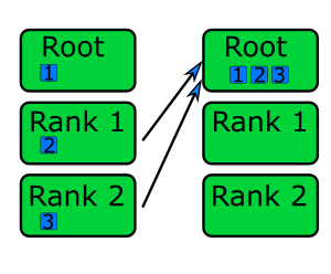
In the code example below, MPI_Gather() is used to gather the contents of rank_data from each rank, to rank 0 (the
root rank).
int rank_data[NUM_DATA_POINTS];

/* Each rank generates some data, including the root rank */
for (int i = 0; i < NUM_DATA_POINTS; ++i) {
    rank_data[i] = (rank + 1) * (i + 1);
}

/* To gather all of the data, we need a buffer to store it. To make sure we have enough
   space, we need to make sure we allocate enough memory on the root rank */
int recv_count = NUM_DATA_POINTS * num_ranks;
int *gathered_data = malloc(recv_count * sizeof(int));

/* MPI_Gather is used in a similar way to MPI_Scatter. Note how that even though we have
   allocated recv_count elements for *gathered_data, MPI_Gather has recv_count set to
   NUM_DATA_POINTS. This is because we are expecting to receive that many elements from
   each rank */
MPI_Gather(rank_data, NUM_DATA_POINTS, MPI_INT, gathered_data, NUM_DATA_POINTS, MPI_INT, 0, MPI_COMM_WORLD);
Gathering greetings
In the previous episode, we used point-to-point communication to send a greeting message to rank 0 from every other rank. Instead of using point-to-point communication functions, re-implement your solution using
MPI_Gather()instead. You can use this code as your starting point.Solution
#include <mpi.h>
#include <stdio.h>
#include <stdlib.h>

#define NUM_CHARS 32

int main(int argc, char **argv) {
    int my_rank, num_ranks;
    MPI_Init(&argc, &argv);
    MPI_Comm_rank(MPI_COMM_WORLD, &my_rank);
    MPI_Comm_size(MPI_COMM_WORLD, &num_ranks);

    char message[NUM_CHARS];
    snprintf(message, NUM_CHARS, "Hello from rank %d", my_rank);

    char *recv_buffer = malloc(NUM_CHARS * num_ranks * sizeof(char));
    MPI_Gather(message, NUM_CHARS, MPI_CHAR, recv_buffer, NUM_CHARS, MPI_CHAR, 0, MPI_COMM_WORLD);

    if (my_rank == 0) {
        for (int i = 0; i < num_ranks; ++i) { // snprintf null terminates strings
            printf("%s\n", &recv_buffer[i * NUM_CHARS]);
        }
    }

    free(recv_buffer);

    return MPI_Finalize();
}
Reduce
A reduction operation is one which takes a values across the ranks, and combines them into a single value. Reductions
are probably the most common collective operation you will use. The example at the beginning of this episode was a
reduction operation, summing up a bunch of numbers, implemented using point-to-point communication. Reduction operations
can be done using the collection function MPI_Reduce(), which has the following arguments,
int MPI_Reduce(
    void *sendbuf,
    void *recvbuffer,
    int count,
    MPI_Datatype datatype,
    MPI_Op op,
    int root,
    MPI_Comm comm
);
*sendbuf: |
The data to be reduced by the root rank |
*recvbuf: |
A buffer to contain the reduction output |
count: |
The number of elements of data to be reduced |
datatype: |
The data type of the data |
op: |
The reduction operation to perform |
root: |
The root rank, which will perform the reduction |
comm: |
The communicator |
The op argument controls which reduction operation is carried out, from the following possible operations:
| Operation | Description |
|---|---|
MPI_SUM |
Calculate the sum of numbers sent by each rank. |
MPI_MAX |
Return the maximum value of numbers sent by each rank. |
MPI_MIN |
Return the minimum of numbers sent by each rank. |
MPI_PROD |
Calculate the product of numbers sent by each rank. |
MPI_MAXLOC |
Return the maximum value and the number of the rank that sent the maximum value. |
MPI_MINLOC |
Return the minimum value of the number of the rank that sent the minimum value. |
In a reduction operation, each ranks sends a piece of data to the root rank, which are combined, depending on the choice of operation, into a single value on the root rank, as shown in the diagram below. Since the data is sent and operation done on the root rank, it means the reduced value is only available on the root rank.
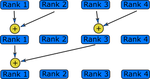
By using MPI_Reduce() and MPI_Bcast(), we can refactor the first code example into two collective functions,
MPI_Comm_rank(MPI_COMM_WORLD, &my_rank);

int sum;
MPI_Reduce(&my_rank, &sum, 1, MPI_INT, MPI_SUM, 0, MPI_COMM_WORLD);
MPI_Bcast(&sum, 1, MPI_INT, 0, MPI_COMM_WORLD);  /* Using MPI_Bcast to send the reduced value to every rank */
All-to-All
Allreduce
In the code example just above, after the reduction operation we used MPI_Bcast() to communicate the result to every
rank in the communicator. This is a common pattern, so much so that there is a collective operation which does both in a
single function call,
int MPI_Allreduce(
    void *sendbuf,          /* The data to be reduced */
    void *recvbuffer,       /* The buffer which will contain the reduction output */
    int count,              /* The number of elements of data to be reduced */
    MPI_Datatype datatype,  /* The data type of the data */
    MPI_Op op,              /* The reduction operation to use */
    MPI_Comm comm           /* The communicator where the reduction will be performed */
);
*sendbuf: |
The data to be reduced, on all ranks |
*recvbuf: |
A buffer which will contain the reduction output |
count: |
The number of elements of data to be reduced |
datatype: |
The data type of the data |
op: |
The reduction operation to use |
comm: |
The communicator |
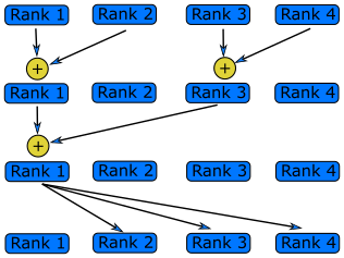
MPI_Allreduce() performs the same operations as MPI_Reduce(), but the result is sent to all ranks rather than only
being available on the root rank. This means we can remove the MPI_Bcast() in the previous code example and remove
almost all of the code in the reduction example using point-to-point communication at the beginning of the episode. This
is shown in the following code example.
int sum;
MPI_Comm_rank(MPI_COMM_WORLD, &my_rank);

/* MPI_Allreduce effectively replaces all of the code in the first example of this
   episode, and is also faster */
MPI_Allreduce(&my_rank, &sum, 1, MPI_INT, MPI_SUM, MPI_COMM_WORLD);
In-place operations
In MPI, we can use in-place operations to eliminate the need for separate send and receive buffers in some collective operations. We typically do this by using the
MPI_IN_PLACEconstant in place of the send buffer, as in the example below usingMPI_Allreduce().sum = my_rank; MPI_Allreduce(MPI_IN_PLACE, &sum, 1, MPI_INT, MPI_SUM, 0, MPI_COMM_WORLD);Not all collective operations support in-place operations, and the usage of
MPI_IN_PLACEcan be different for the other collective functions which support it.
Reductions
The following program creates an array called
vectorthat contains a list ofn_numberson each rank. The first rank contains the numbers from 1 to n_numbers, the second rank from n_numbers to 2*n_numbers and so on. It then calls thefind_maxandfind_sumfunctions that should calculate the sum and maximum of the vector.These functions are not implemented in parallel and only return the sum and the maximum of the local vectors. Modify the
find_sumandfind_maxfunctions to work correctly in parallel usingMPI_ReduceorMPI_Allreduce.#include <stdio.h> #include <mpi.h> // Calculate the sum of numbers in a vector double find_sum(double * vector, int N) { double sum = 0; for (int i = 0; i < N; ++i){ sum += vector[i]; } return sum; } // Find the maximum of numbers in a vector double find_maximum(double *vector, int N) { double max = 0; for (int i = 0; i < N; ++i){ if (vector[i] > max){ max = vector[i]; } } return max; } int main(int argc, char **argv) { int n_numbers = 1024; int rank; double vector[n_numbers]; double sum, max; double my_first_number; // First call MPI_Init MPI_Init(&argc, &argv); // Get my rank MPI_Comm_rank(MPI_COMM_WORLD, &rank); // Each rank will have n_numbers numbers, // starting from where the previous left off my_first_number = n_numbers*rank; // Generate a vector for (int i = 0; i < n_numbers; ++i) { vector[i] = my_first_number + i; } //Find the sum and print sum = find_sum( vector, n_numbers ); printf("The sum of the numbers is %f\n", sum); //Find the maximum and print max = find_maximum( vector, n_numbers ); printf("The largest number is %f\n", max); // Call finalize at the end return MPI_Finalize(); }Solution
// Calculate the sum of numbers in a vector
double find_sum(double *vector, int N) {
   double sum = 0;
   double global_sum;

   // Calculate the sum on this rank as before
   for (int i = 0; i < N; ++i){
      sum += vector[i];
   }

   // Call MPI_Allreduce to find the full sum
   MPI_Allreduce(&sum, &global_sum, 1, MPI_DOUBLE, MPI_SUM, MPI_COMM_WORLD);

   return global_sum;
}

// Find the maximum of numbers in a vector
double find_maximum(double *vector, int N) {
   double max = 0;
   double global_max;

   // Calculate the sum on this rank as before
   for (int i = 0; i < N; ++i){
      if (vector[i] > max){
         max = vector[i];
      }
   }

   // Call MPI_Allreduce to find the maximum over all the ranks
   MPI_Allreduce(&max, &global_max, 1, MPI_DOUBLE, MPI_MAX, MPI_COMM_WORLD);

   return global_max;
}
More collective operations are available
The collective functions introduced in this episode do not represent an exhaustive list of all collective operations in MPI. There are a number which are not covered, as their usage is not as common. You can usually find a list of the collective functions available for the implementation of MPI you choose to use, e.g. Microsoft MPI documentation .
Key Points
Using point-to-point communication to send/receive data to/from all ranks is inefficient
It’s far more efficient to send/receive data to/from multiple ranks by using collective operations
Non-blocking Communication
Overview
Teaching: 15 min
Exercises: 20 minQuestions
What are the advantages of non-blocking communication?
How do I use non-blocking communication?
Objectives
Describe the advantages and disadvantages of non-blocking communication
Use non-blocking variants of MPI’s send and receive functions
Use MPI to wait until a non-blocking MPI communication has completed
Use MPI to test the status of non-blocking MPI communication
Use non-blocking variants of MPI’s collective functions
In the previous episodes, we learnt how to send messages between two ranks or collectively to multiple ranks. In both cases, we used blocking communication functions which meant our program wouldn’t progress until the communication had completed. It takes time and computing power to transfer data into buffers, to send that data around (over the network) and to receive the data into another rank. But for the most part, the CPU isn’t actually doing much at all during communication, when it could still be number crunching.
Why bother with non-blocking communication?
Non-blocking communication is communication which happens in the background. So we don’t have to let any CPU cycles go to waste! If MPI is dealing with the data transfer in the background, we can continue to use the CPU in the foreground and keep doing tasks whilst the communication completes. By overlapping computation with communication, we hide the latency/overhead of communication. This is critical for lots of HPC applications, especially when using lots of CPUs, because, as the number of CPUs increases, the overhead of communicating with them all also increases. If you use blocking synchronous sends, the time spent communicating data may become longer than the time spent creating data to send! All non-blocking communications are asynchronous, even when using synchronous sends, because the communication happens in the background, even though the communication cannot complete until the data is received.
So, how do I use non-blocking communication?
Just as with buffered, synchronous, ready and standard sends, MPI has to be programmed to use either blocking or non-blocking communication. For almost every blocking function, there is a non-blocking equivalent. They have the same name as their blocking counterpart, but prefixed with “I”. The “I” stands for “immediate”, indicating that the function returns immediately and does not block the program. The table below shows some examples of blocking functions and their non-blocking counterparts.
Blocking Non-blocking MPI_Bsend()MPI_Ibsend()MPI_Barrier()MPI_Ibarrier()MPI_Reduce()MPI_Ireduce()But, this isn’t the complete picture. As we’ll see later, we need to do some additional bookkeeping to be able to use non-blocking communications.
By effectively utilizing non-blocking communication, we can develop applications that scale significantly better during intensive communication. However, this comes with the trade-off of both increased conceptual and code complexity. Since non-blocking communication doesn’t keep control until the communication finishes, we don’t actually know if a communication has finished unless we check; this is usually referred to as synchronisation, as we have to keep ranks in sync to ensure they have the correct data. So whilst our program continues to do other work, it also has to keep pinging to see if the communication has finished, to ensure ranks are synchronised. If we check too often, or don’t have enough tasks to “fill in the gaps”, then there is no advantage to using non-blocking communication and we may replace communication overheads with time spent keeping ranks in sync! It is not always clear cut or predictable if non-blocking communication will improve performance. For example, if one ranks depends on the data of another, and there are no tasks for it to do whilst it waits, that rank will wait around until the data is ready, as illustrated in the diagram below. This essentially makes that non-blocking communication a blocking communication. Therefore unless our code is structured to take advantage of being able to overlap communication with computation, non-blocking communication adds complexity to our code for no gain.
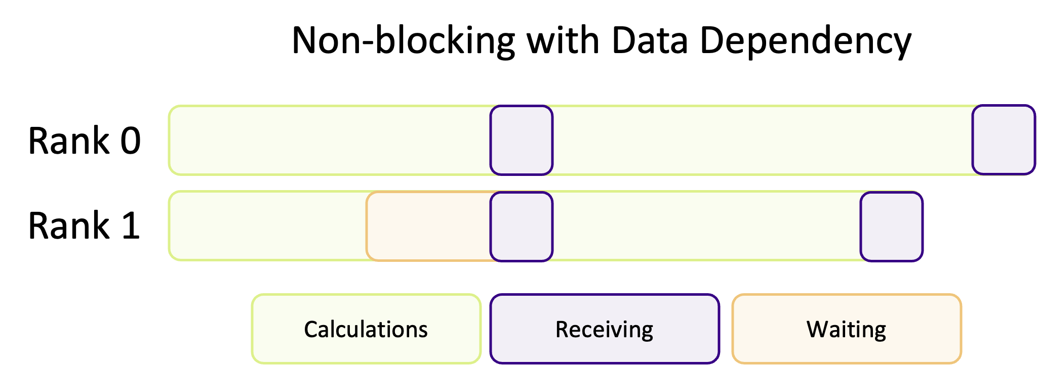
Advantages and disadvantages
What are the main advantages of using non-blocking communication, compared to blocking? What about any disadvantages?
Solution
Some of the advantages of non-blocking communication over blocking communication include:
- Non-blocking communication gives us the ability to interleave communication with computation. By being able to use the CPU whilst the network is transmitting data, we create algorithms with more efficient hardware usage.
- Non-blocking communication also improve the scalability of our program, due to the smaller communication overhead and latencies associated with communicating between a large number of ranks.
- Non-blocking communication is more flexible, which allows for more sophisticated parallel and communication algorithms.
On the other hand, some disadvantages are:
- It is more difficult to use non-blocking communication. Not only does it result in more, and more complex, lines of code, we also have to worry about rank synchronisation and data dependency.
- Whilst typically using non-blocking communication, where appropriate, improves performance, it’s not always clear cut or predictable if non-blocking will result in sufficient performance gains to justify the increased complexity.
Point-to-point communication
For each blocking communication function we’ve seen, a non-blocking variant exists. For example, if we take
MPI_Send(), the non-blocking variant is MPI_Isend() which has the arguments,
int MPI_Isend(
    void *buf,
    int count,
    MPI_Datatype datatype,
    int dest,
    int tag,
    MPI_Comm comm,
    MPI_Request *request
);
*buf: |
The data to be sent |
count: |
The number of elements of data |
datatype: |
The data types of the data |
dest: |
The rank to send data to |
tag: |
The communication tag |
comm: |
The communicator |
*request: |
The request handle, used to track the communication |
The arguments are identical to MPI_Send(), other than the addition of the *request argument. This argument is known
as an handle (because it “handles” a communication request) which is used to track the progress of a (non-blocking)
communication.
When we use non-blocking communication, we have to follow it up with MPI_Wait() to synchronise the
program and make sure *buf is ready to be re-used. This is incredibly important to do. Suppose we are sending an array
of integers,
MPI_Isend(some_ints, 5, MPI_INT, 1, 0, MPI_COMM_WORLD, &request);
some_ints[1] = 5;  /* !!! don't do this !!! */
Modifying some_ints before the send has completed is undefined behaviour, and can result in breaking results! For
example, if MPI_Isend decides to use its buffered mode then modifying some_ints before it’s finished being copied to
the send buffer will means the wrong data is sent. Every non-blocking communication has to have a corresponding
MPI_Wait(), to wait and synchronise the program to ensure that the data being sent is ready to be modified again.
MPI_Wait() is a blocking function which will only return when a communication has finished.
int MPI_Wait(
    MPI_Request *request,
    MPI_Status *status
);
*request: |
The request handle for the communication |
*status: |
The status handle for the communication |
Once we have used MPI_Wait() and the communication has finished, we can safely modify some_ints again. To receive
the data send using a non-blocking send, we can use either the blocking MPI_Recv() or it’s non-blocking variant,
int MPI_Irecv(
    void *buf,              /* The buffer to receive data into */
    int count,              /* The number of elements of data to receive */
    MPI_Datatype datatype,  /* The datatype of the data being received */
    int source,             /* The rank to receive data from */
    int tag,                /* The communication tag */
    MPI_Comm comm,          /* The communicator to use */
    MPI_Request *request,   /* The communication request handle */
);
*buf: |
A buffer to receive data into |
count: |
The number of elements of data to receive |
datatype: |
The data type of the data |
source: |
The rank to receive data from |
tag: |
The communication tag |
comm: |
The communicator |
*request: |
The request handle for the receive |
True or false?
Is the following statement true or false? Non-blocking communication guarantees immediate completion of data transfer.
Solution
False. Just because the communication function has returned, does not mean the communication has finished and the communication buffer is ready to be re-used or read from. Before we access, or edit, any data which has been used in non-blocking communication, we always have to test/wait for the communication to finish using
MPI_Wait()before it is safe to use it.
In the example below, an array of integers (some_ints) is sent from rank 0 to rank 1 using non-blocking communication.
MPI_Status status;
MPI_Request request;

int recv_ints[5];
int some_ints[5] = { 1, 2, 3, 4, 5 };

if (my_rank == 0) {
    MPI_Isend(some_ints, 5, MPI_INT, 1, 0, MPI_COMM_WORLD, &request);
    MPI_Wait(&request, &status);
    some_ints[1] = 42;  // After MPI_Wait(), some_ints has been sent and can be modified again
} else {
    MPI_Irecv(recv_ints, 5, MPI_INT, 0, 0, MPI_COMM_WORLD, &request);
    MPI_Wait(&request, &status);
    int data_i_wanted = recv_ints[2];  // recv_ints isn't guaranteed to have the correct data until after MPI_Wait()
}
The code above is functionally identical to blocking communication, because of MPI_Wait() is blocking. The program
will not continue until MPI_Wait() returns. Since there is no additional work between the communication call and
blocking wait, this is a poor example of how non-blocking communication should be used. It doesn’t take advantage of the
asynchronous nature of non-blocking communication at all. To really make use of non-blocking communication, we need to
interleave computation (or any busy work we need to do) with communication, such as as in the next example.
MPI_Status status;
MPI_Request request;

if (my_rank == 0) {
    // This send important_data without being blocked and move into the next work
    MPI_Isend(important_data, 16, MPI_INT, 1, 0, MPI_COMM_WORLD, &request);
} else {
    // Start listening for the message from the other rank, but isn't blocked
    MPI_Irecv(important_data, 16, MPI_INT, 0, 0, MPI_COMM_WORLD, &request);
}

// Whilst the message is still sending or received, we should do some other work
// to keep using the CPU (which isn't required for most of the communication.
// IMPORTANT: the work here cannot modify or rely on important_data */
clear_model_parameters();
initialise_model();

// Once we've done the work which doesn't require important_data, we need to wait until the
// data is sent/received if it hasn't already */
MPI_Wait(&request, &status);

// Now the model is ready and important_data has been sent/received, the simulation
// carries on
simulate_something(important_data);
What about deadlocks?
Deadlocks are easily created when using blocking communication. The code snippet below shows an example of deadlock from one of the previous episodes.
if (my_rank == 0) {
    MPI_Send(&numbers, 8, MPI_INT, 1, 0, MPI_COMM_WORLD);
    MPI_Recv(&numbers, 8, MPI_INT, 1, 0, MPI_COMM_WORLD, &status);
} else {
    MPI_Send(&numbers, 8, MPI_INT, 0, 0, MPI_COMM_WORLD);
    MPI_Recv(&numbers, 8, MPI_INT, 0, 0, MPI_COMM_WORLD, &status);
}
If we changed to non-blocking communication, do you think there would still be a deadlock? Try writing your own non-blocking version.
Solution
The non-blocking version of the code snippet may look something like this:
MPI_Request send_req, recv_req;

if (my_rank == 0) {
    MPI_Isend(numbers, 8, MPI_INT, 1, 0, MPI_COMM_WORLD, &send_req);
    MPI_Irecv(numbers, 8, MPI_INT, 1, 0, MPI_COMM_WORLD, &recv_req);
} else {
    MPI_Isend(numbers, 8, MPI_INT, 0, 0, MPI_COMM_WORLD, &send_req);
    MPI_Irecv(numbers, 8, MPI_INT, 0, 0, MPI_COMM_WORLD, &recv_req);
}

MPI_Status statuses[2];
MPI_Request requests[2] = { send_req, recv_req };
MPI_Waitall(2, requests, statuses);  // Wait for both requests in one function
This version of the code will not deadlock, because the non-blocking functions return immediately. So even though rank 0 and 1 one both send, meaning there is no corresponding receive, the immediate return from send means the receive function is still called. Thus a deadlock cannot happen.
However, it is still possible to create a deadlock using
MPI_Wait(). IfMPI_Wait()is waiting to forMPI_Irecv()to get some data, but there is no matching send operation (so no data has been sent), thenMPI_Wait()can never return resulting in a deadlock. In the example code below, rank 0 becomes deadlocked.MPI_Status status; MPI_Request send_req, recv_req; if (my_rank == 0) { MPI_Isend(numbers, 8, MPI_INT, 1, 0, MPI_COMM_WORLD, &send_req); MPI_Irecv(numbers, 8, MPI_INT, 1, 0, MPI_COMM_WORLD, &recv_req); } else { MPI_Irecv(numbers, 8, MPI_INT, 0, 0, MPI_COMM_WORLD, &recv_req); } MPI_Wait(&send_req, &status); MPI_Wait(&recv_req, &status); // Wait for both requests in one function
To wait, or not to wait
In some sense, by using MPI_Wait() we aren’t fully non-blocking because we still block execution whilst we wait for
communications to complete. To be “truly” asynchronous we can use another function called MPI_Test() which, at face
value, is the non-blocking counterpart of MPI_Wait(). When we use MPI_Test(), it checks if a communication is
finished and sets the value of a flag to true if it is and returns. If a communication hasn’t finished, MPI_Test()
still returns but the value of the flag is false instead. MPI_Test() has the following arguments,
int MPI_Test(
    MPI_Request *request,
    int *flag,
    MPI_Status *status,
);
*request: |
The request handle for the communication |
*flag: |
A flag to indicate if the communication has completed |
*status: |
The status handle for the communication |
*request and *status are the same you’d use for MPI_Wait(). *flag is the variable which is modified to indicate
if the communication has finished or not. Since it’s an integer, if the communication hasn’t finished then flag == 0.
We use MPI_Test() is much the same way as we’d use MPI_Wait(). We start a non-blocking communication, and keep doing
other, independent, tasks whilst the communication finishes. The key difference is that since MPI_Test() returns
immediately, we may need to make multiple calls before the communication is finished. In the code example below,
MPI_Test() is used within a while loop which keeps going until either the communication has finished or until
there is no other work left to do.
MPI_Status status;
MPI_Request request;
MPI_Irecv(recv_buffer, 16, MPI_INT, 0, 0, MPI_COMM_WORLD, &request);

// We need to define a flag, to track when the communication has completed
int comm_completed = 0;

// One example use case is keep checking if the communication has finished, and continuing
// to do CPU work until it has
while (!comm_completed && work_still_to_do()) {
    do_some_other_work();
    // MPI_Test will return flag == true when the communication has finished
    MPI_Test(&request, &comm_completed, &status);
}

// If there is no more work and the communication hasn't finished yet, then we should wait
// for it to finish
if (!comm_completed) {
    MPI_Wait(&request, &status);
}
Dynamic task scheduling
Dynamic task schedulers are a class of algorithms designed to optimise the work load across ranks. The most efficient, and, really, only practical, implementations use non-blocking communication to periodically check the work balance and asynchronously assign and send additional work to a rank, in the background, as it continues to work on its current queue of work.
An interesting aside: communication timeouts
Non-blocking communication gives us a lot of flexibility, letting us write complex communication algorithms to experiment and find the right solution. One example of that flexibility is using
MPI_Test()to create a communication timeout algorithm.#define COMM_TIMEOUT 60 // seconds clock_t start_time = clock(); double elapsed_time = 0.0; int comm_completed = 0 while (!comm_completed && elapsed_time < COMM_TIMEOUT) { // Check if communication completed MPI_Test(&request, &comm_completed, &status); // Update elapsed time elapsed_time = (double)(clock() - start_time) / CLOCKS_PER_SEC; } if (elapsed_time >= COMM_TIMEOUT) { MPI_Cancel(&request); // Cancel the request to stop the, e.g. receive operation handle_communication_errors(); // Put the program into a predictable state }Something like this would effectively remove deadlocks in our program, and allows us to take appropriate actions to recover the program back into a predictable state. In reality, however, it would be hard to find a useful and appropriate use case for this in scientific computing. In any case, though, it demonstrate the power and flexibility offered by non-blocking communication.
Try it yourself
In the MPI program below, a chain of ranks has been set up so one rank will receive a message from the rank to its left and send a message to the one on its right, as shown in the diagram below:
For following skeleton below, use non-blocking communication to send
send_messageto the right right and receive a message from the left rank. Create two programs, one usingMPI_Wait()and the other usingMPI_Test().#include <mpi.h> #include <stdio.h> #define MESSAGE_SIZE 32 int main(int argc, char **argv) { int my_rank; int num_ranks; MPI_Init(&argc, &argv); MPI_Comm_rank(MPI_COMM_WORLD, &my_rank); MPI_Comm_size(MPI_COMM_WORLD, &num_ranks); if (num_ranks < 2) { printf("This example requires at least two ranks\n"); MPI_Abort(MPI_COMM_WORLD, 1); } char send_message[MESSAGE_SIZE]; char recv_message[MESSAGE_SIZE]; int right_rank = (my_rank + 1) % num_ranks; int left_rank = my_rank < 1 ? num_ranks - 1 : my_rank - 1; sprintf(send_message, "Hello from rank %d!", my_rank); // Your code goes here return MPI_Finalize(); }The output from your program should look something like this:
Rank 0: message received -- Hello from rank 3!
Rank 1: message received -- Hello from rank 0!
Rank 2: message received -- Hello from rank 1!
Rank 3: message received -- Hello from rank 2!
Solution
Note that in the solution below, we started listening for the message before
send_messageeven had its message ready!#include <mpi.h> #include <stdbool.h> #include <stdio.h> #define MESSAGE_SIZE 32 int main(int argc, char **argv) { int my_rank; int num_ranks; MPI_Init(&argc, &argv); MPI_Comm_rank(MPI_COMM_WORLD, &my_rank); MPI_Comm_size(MPI_COMM_WORLD, &num_ranks); if (num_ranks < 2) { printf("This example requires at least two ranks\n"); return MPI_Finalize(); } char send_message[MESSAGE_SIZE]; char recv_message[MESSAGE_SIZE]; int right_rank = (my_rank + 1) % num_ranks; int left_rank = my_rank < 1 ? num_ranks - 1 : my_rank - 1; MPI_Status send_status, recv_status; MPI_Request send_request, recv_request; MPI_Irecv(recv_message, MESSAGE_SIZE, MPI_CHAR, left_rank, 0, MPI_COMM_WORLD, &recv_request); sprintf(send_message, "Hello from rank %d!", my_rank); MPI_Isend(send_message, MESSAGE_SIZE, MPI_CHAR, right_rank, 0, MPI_COMM_WORLD, &send_request); MPI_Wait(&send_request, &send_status); MPI_Wait(&recv_request, &recv_status); /* But maybe you prefer MPI_Test() int recv_flag = false; while (recv_flag == false) { MPI_Test(&recv_request, &recv_flag, &recv_status); } */ printf("Rank %d: message received -- %s\n", my_rank, recv_message); return MPI_Finalize(); }
Collective communication
Since the release of MPI 3.0, the collective operations have non-blocking versions. Using these non-blocking collective
operations is as easy as we’ve seen for point-to-point communication in the last section. If we want to do a
non-blocking reduction, we’d use MPI_Ireduce(),
int MPI_Ireduce(
    const void *sendbuf,
    void *recvbuf,
    int count,
    MPI_Datatype datatype,
    MPI_Op op,
    int root,
    MPI_Comm comm,
    MPI_Request *request,
);
*sendbuf: |
The data to be reduced by the root rank |
*recvbuf: |
A buffer to contain the reduction output |
count: |
The number of elements of data to be reduced |
datatype: |
The data type of the data |
op: |
The reduction operation to perform |
root: |
The root rank, which will perform the reduction |
comm: |
The communicator |
*request: |
The request handle for the communicator |
As with MPI_Send() vs. MPI_Isend() the only change in using the non-blocking variant of MPI_Reduce() is the
addition of the *request argument, which returns a request handle. This is the request handle we’ll use with either
MPI_Wait() or MPI_Test() to ensure that the communication has finished, and been successful. The below code examples
shows a non-blocking reduction,
MPI_Status status;
MPI_Request request;

int recv_data;
int send_data = my_rank + 1;

/* MPI_Iallreduce is the non-blocking version of MPI_Allreduce. This reduction operation will sum send_data
   for all ranks and distribute the result back to all ranks into recv_data */
MPI_Iallreduce(&send_data, &recv_data, 1, MPI_INT, MPI_SUM, MPI_COMM_WORLD, &request);
/* Remember, using MPI_Wait() straight after the communication is equivalent to using a blocking communication */
MPI_Wait(&request, &status);
What’s
MPI_Ibarrier()all about?In the previous episode, we learnt that
MPI_Barrier()is a collective operation we can use to bring all the ranks back into synchronisation with one another. How do you think the non-blocking variant,MPI_Ibarrier(), is used and how might you use this in your program? You may want to read the relevant documentation first.Solution
When a rank reaches a non-blocking barrier,
MPI_Ibarrier()will return immediately whether other ranks have reached the barrier or not. The behaviour of the barrier we would expect is enforced at the nextMPI_Wait()(orMPI_Test()) operation.MPI_Wait()will return once all the ranks have reached the barrier.Non-blocking barriers can be used to help hide/reduce synchronisation overhead. We may want to add a synchronisation point in our program so the ranks start some work all at the same time. With a blocking barrier, the ranks have to wait for every rank to reach the barrier, and can’t do anything other than wait. But with a non-blocking barrier, we can overlap the barrier operation with other, independent, work whilst ranks wait for the other ranks to catch up.
Reduce and broadcast
Using non-blocking collective communication, calculate the sum of
my_num = my_rank + 1from each MPI rank and broadcast the value of the sum to every rank. To calculate the sum, use eitherMPI_Igather()orMPI_Ireduce(). You should use the code below as your starting point.#include <mpi.h> #include <stdio.h> int main(int argc, char **argv) { int my_rank; int num_ranks; MPI_Init(&argc, &argv); MPI_Comm_rank(MPI_COMM_WORLD, &my_rank); MPI_Comm_size(MPI_COMM_WORLD, &num_ranks); if (num_ranks < 2) { printf("This example needs at least 2 ranks\n"); MPI_Finalize(); return 1; } int sum = 0; int my_num = my_rank + 1; printf("Start : Rank %d: my_num = %d sum = %d\n", my_rank, my_num, sum); // Your code goes here printf("End : Rank %d: my_num = %d sum = %d\n", my_rank, my_num, sum); return MPI_Finalize(); }For two ranks, the output should be:
Start : Rank 0: my_num = 1 sum = 0
Start : Rank 1: my_num = 2 sum = 0
End : Rank 0: my_num = 1 sum = 3
End : Rank 1: my_num = 2 sum = 3
Solution
The solution below uses
MPI_Irduce()to calculate the sum andMPI_Ibcast()to broadcast it to all ranks. For an even shorter solution,MPI_Ireduceall()would also achieve the same thing in a single line!int main(int argc, char **argv) { int my_rank; int num_ranks; MPI_Init(&argc, &argv); MPI_Comm_rank(MPI_COMM_WORLD, &my_rank); MPI_Comm_size(MPI_COMM_WORLD, &num_ranks); if (num_ranks < 2) { printf("This example needs at least 2 ranks\n"); MPI_Finalize(); return 1; } int sum = 0; int my_num = my_rank + 1; printf("Start : Rank %d: my_num = %d sum = %d\n", my_rank, my_num, sum); MPI_Status status; MPI_Request request; MPI_Ireduce(&my_num, &sum, 1, MPI_INT, MPI_SUM, 0, MPI_COMM_WORLD, &request); MPI_Wait(&request, &status); MPI_Ibcast(&sum, 1, MPI_INT, 0, MPI_COMM_WORLD, &request); MPI_Wait(&request, &status); printf("End : Rank %d: my_num = %d sum = %d\n", my_rank, my_num, sum); return MPI_Finalize(); }
Key Points
Non-blocking communication often leads to performance improvements compared to blocking communication
However, it is usually more difficult to use non-blocking communication
Most blocking communication operations have a non-blocking variant
We have to wait for a communication to finish using
MPI_Wait()(orMPI_Test()) otherwise we will encounter strange behaviour
Derived Data Types
Overview
Teaching: 25 min
Exercises: 20 minQuestions
How do I use complex data structures in MPI?
What is contiguous memory, and why does it matter?
Objectives
Explain what a derived data type is and how they can help
Define and explain the challenges associated with non-contiguous memory
Describe the limitations of using malloc() in terms of memory contiguity
Use vectors to send column slices of an array to another rank
We’ve so far seen the basic building blocks for splitting work and communicating data between ranks, meaning we’re now dangerous enough to write a simple and successful MPI application. We’ve worked, so far, with simple data structures, such as single variables or small 1D arrays. In reality, any useful software we write will use more complex data structures, such as n-dimensional arrays, structures and other complex types. Working with these in MPI require a bit more work to communicate them correctly and efficiently.
To help with this, MPI provides an interface to create new types known as derived data types. A derived type acts as a way to enable the translation of complex data structures into instructions which MPI uses for efficient data access communication. In this episode, we will learn how to use derived data types to send array vectors and sub-arrays.
Size limitations for messages
All throughout MPI, the argument which says how many elements of data are being communicated is an integer:
int
count
. In most 64-bit Linux systems,int’s are usually 32-bit and so the biggest number you can pass tocountis2^31 - 1 = 2,147,483,647, which is about 2 billion. Arrays which exceed this length can’t be communicated easily in versions of MPI older than MPI-4.0, when support for “large count” communication was added to the MPI standard. In older MPI versions, there are two workarounds to this limitation. The first is to communicate large arrays in smaller, more manageable chunks. The other is to use derived types, to re-shape the data.
Almost all scientific and computing problems nowadays require us to think in more than one dimension. Using multi-dimensional arrays, such for matrices or tensors, or discretising something onto a 2D or 3D grid of points are fundamental parts of a lot of software. However, the additional dimensions comes with additional complexity, not just in the code we write, but also in how data is communicated.
To create a 2 x 3 matrix, in C, and initialize it with some values, we use the following syntax,
int matrix[2][3] = { {1, 2, 3}, {4, 5, 6} }; // matrix[rows][cols]
This creates an array with two rows and three columns. The first row contains the values {1, 2, 3} and the second row
contains {4, 5, 6}. The number of rows and columns can be any value, as long as there is enough memory available.
The importance of memory contiguity
When a sequence of things is contiguous, it means there are multiple adjacent things without anything in between them. In the context of MPI, when we talk about something being contiguous we are almost always talking about how arrays, and other complex data structures, are stored in the computer’s memory. The elements in an array are contiguous when the next and previous elements are stored in adjacent memory locations.
The memory space of a computer is linear. When we create a multi-dimensional array, the compiler and operating system
decide how to map and store the elements onto that linear space. There are two ways to do this:
row-major or column-major. The difference
is which elements of the array are contiguous in memory. Arrays are row-major in C and column-major in Fortran.
In a row-major array, the elements in each column of a row are contiguous, so element x[i][j] is
preceded by x[i][j - 1] and is followed by x[i][j +1]. In Fortran, arrays are column-major so x(i, j) is
followed by x(i + 1, j) and so on.
The diagram below shows how a 4 x 4 matrix is mapped onto a linear memory space, for a row-major array. At the top of the diagram is the representation of the linear memory space, where each number is ID of the element in memory. Below that are two representations of the array in 2D: the left shows the coordinate of each element and the right shows the ID of the element.
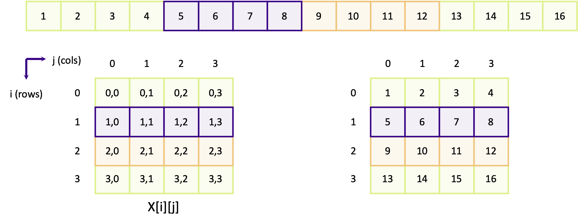
The purple elements (5, 6, 7, 8) which map to the coordinates [1][0], [1][1], [1][2] and [1][3] are contiguous
in linear memory. The same applies for the orange boxes for the elements in row 2 (elements 9, 10, 11 and 12). Columns
in row-major arrays are contiguous. The next diagram instead shows how elements in adjacent rows are mapped in memory.
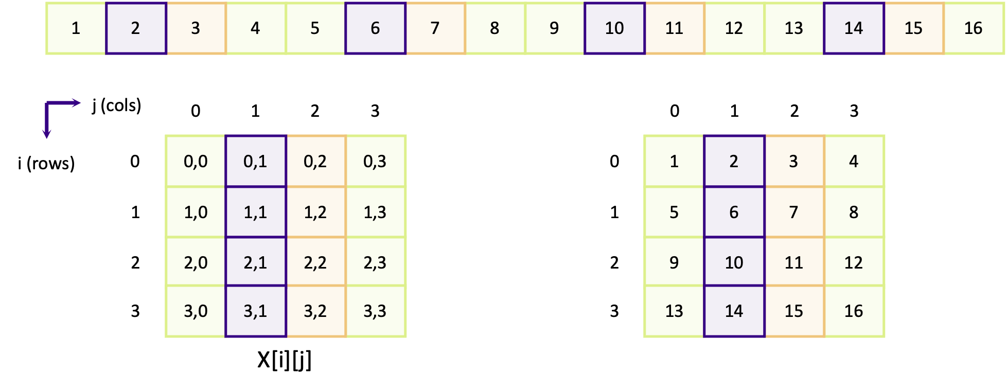
Looking first at the purple boxes (containing elements 2, 6, 10 and 14) which make up the row elements for column 1,
we can see that the elements are not contiguous. Element [0][1] maps to element 2 and element [1][1] maps to element
6 and so on. Elements in the same column but in a different row are separated by four other elements, in this example.
In other words, elements in other rows are not contiguous.
Does memory contiguity affect performance?
Do you think memory contiguity could impact the performance of our software, in a negative way?
Solution
Yes, memory contiguity can affect how fast our programs run. When data is stored in a neat and organized way, the computer can find and use it quickly. But if the data is scattered around randomly (fragmented), it takes more time to locate and use it, which decreases performance. Keeping our data and data access patterns organized can make our programs faster. But we probably won’t notice the difference for small arrays and data structures.
What about if I use
malloc()?More often than not we will see
malloc()being used to allocate memory for arrays. Especially if the code is using an older standard, such as C90, which does not support variable length arrays. When we usemalloc(), we get a contiguous array of elements. To create a 2D array usingmalloc(), we have to first create an array of pointers (which are contiguous) and allocate memory for each pointer,int num_rows = 3, num_cols = 5; float **matrix = malloc(num_rows * sizeof(float*)); // Each pointer is the start of a row for (int i = 0; i < num_rows; ++i) { matrix[i] = malloc(num_cols * sizeof(float)); // Here we allocate memory to store the column elements for row i } for (int i = 0; i < num_rows; ++i) { for (int j = 0; i < num_cols; ++j) { matrix[i][j] = 3.14159; // Indexing is done as matrix[rows][cols] } }There is one problem though.
malloc()does not guarantee that subsequently allocated memory will be contiguous. Whenmalloc()requests memory, the operating system will assign whatever memory is free. This is not always next to the block of memory from the previous allocation. This makes life tricky, since data has to be contiguous for MPI communication. But there are workarounds. One is to only use 1D arrays (with the same number of elements as the higher dimension array) and to map the n-dimensional coordinates into a linear coordinate system. For example, the element[2][4]in a 3 x 5 matrix would be accessed as,int index_for_2_4 = matrix1d[5 * 2 + 4]; // num_cols * row + colAnother solution is to move memory around so that it is contiguous, such as in this example or by using a more sophisticated function such as
arralloc()function (not part of the standard library) which can allocate arbitrary n-dimensional arrays into a contiguous block.
For a row-major array, we can send the elements of a single row (for a 4 x 4 matrix) easily,
MPI_Send(&matrix[1][0], 4, MPI_INT ...);
The send buffer is &matrix[1][0], which is the memory address of the first element in row 1. As the columns are four
elements long, we have specified to only send four integers. Even though we’re working here with a 2D array, sending a
single row of the matrix is the same as sending a 1D array. Instead of using a pointer to the start of the array, an
address to the first element of the row (&matrix[1][0]) is used instead. It’s not possible to do the same for a column
of the matrix, because the elements down the column are not contiguous.
Using vectors to send slices of an array
To send a column of a matrix or array, we have to use a vector. A vector is a derived data type that represents
multiple (or one) contiguous sequences of elements, which have a regular spacing between them. By using vectors, we can
create data types for column vectors, row vectors or sub-arrays, similar to how we can create slices for Numpy arrays
in Python, all of which can be sent in a single, efficient,
communication. To create a vector, we create a new data type using MPI_Type_vector(),
int MPI_Type_vector(
   int count,
   int blocklength,
   int stride,
   MPI_Datatype oldtype,
   MPI_Datatype *newtype
);
count: |
The number of “blocks” which make up the vector |
blocklength: |
The number of contiguous elements in a block |
stride: |
The number of elements between the start of each block |
oldtype: |
The data type of the elements of the vector, e.g. MPI_INT, MPI_FLOAT |
newtype: |
The newly created data type to represent the vector |
To understand what the arguments mean, look at the diagram below showing a vector to send two rows of a 4 x 4 matrix with a row in between (rows 2 and 4),
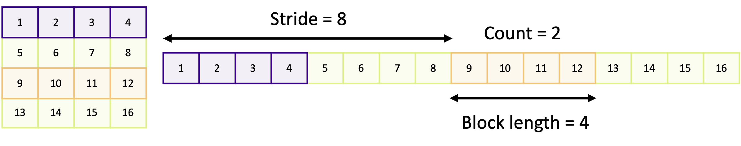
A block refers to a sequence of contiguous elements. In the diagrams above, each sequence of contiguous purple or orange elements represents a block. The block length is the number of elements within a block; in the above this is four. The stride is the distance between the start of each block, which is eight in the example. The count is the number of blocks we want. When we create a vector, we’re creating a new derived data type which includes one or more blocks of contiguous elements.
Why is this functionality useful?
The advantage of using derived types to send vectors is to streamline and simplify communication of complex and non-contiguous data. They are most commonly used where there are boundary regions between MPI ranks, such as in simulations using domain decomposition (see the optional Common Communication Patterns episode for more detail), irregular meshes or composite data structures (covered in the optional Advanced Data Communication episode).
Before we can use the vector we create to communicate data, it has to be committed using MPI_Type_commit(). This
finalises the creation of a derived type. Forgetting to do this step leads to unexpected behaviour, and potentially
disastrous consequences!
int MPI_Type_commit(
   MPI_Datatype *datatype  // The data type to commit - note that this is a pointer
);
When a data type is committed, resources which store information on how to handle it are internally allocated. This
contains data structures such as memory buffers as well as data used for bookkeeping. Failing to free those resources
after finishing with the vector leads to memory leaks, just like when we don’t free memory created using malloc(). To
free up the resources, we use MPI_Type_free(),
int MPI_Type_free (
   MPI_Datatype *datatype  // The data type to clean up -- note this is a pointer
);
The following example code uses a vector to send two rows from a 4 x 4 matrix, as in the example diagram above.
// The vector is a MPI_Datatype
MPI_Datatype rows_type;

// Create the vector type
const int count = 2;
const int blocklength = 4;
const int stride = 8;
MPI_Type_vector(count, blocklength, stride, MPI_INT, &rows_type);

// Don't forget to commit it
MPI_Type_commit(&rows_type);

// Send the middle row of our 2d matrix array. Note that we are sending
// &matrix[1][0] and not matrix. This is because we are using an offset
// to change the starting point of where we begin sending memory
int matrix[4][4] = {
   { 1,  2,  3,  4},
   { 5,  6,  7,  8},
   { 9, 10, 11, 12},
   {13, 14, 15, 16},
};

if (my_rank == 0) {
    MPI_Send(&matrix[1][0], 1, rows_type, 1, 0, MPI_COMM_WORLD);
} else {
    // The receive function doesn't "work" with vector types, so we have to
    // say that we are expecting 8 integers instead
    const int num_elements = count * blocklength;
    int recv_buffer[num_elements];
    MPI_Recv(recv_buffer, num_elements, MPI_INT, 0, 0, MPI_COMM_WORLD, MPI_STATUS_IGNORE);
}

// The final thing to do is to free the new data type when we no longer need it
MPI_Type_free(&rows_type);
There are two things above, which look quite innocent, but are important to understand. First of all, the send buffer
in MPI_Send() is not matrix but &matrix[1][0]. In MPI_Send(), the send buffer is a pointer to the memory
location where the start of the data is stored. In the above example, the intention is to only send the second and forth
rows, so the start location of the data to send is the address for element [1][0]. If we used matrix, the first and
third rows would be sent instead.
The other thing to notice, which is not immediately clear why it’s done this way, is that the receive data type is
MPI_INT and the count is num_elements = count * blocklength instead of a single element of rows_type. This
is because when a rank receives data, the data is contiguous array. We don’t need to use a vector to describe the layout
of contiguous memory. We are just receiving a contiguous array of num_elements = count * blocklength integers.
Sending columns from an array
Create a vector type to send a column in the following 2 x 3 array:
int matrix[2][3] = {
    {1, 2, 3},
    {4, 5, 6},
 };
With that vector type, send the middle column of the matrix (elements
matrix[0][1]andmatrix[1][1]) from rank 0 to rank 1 and print the results. You may want to use this code as your starting point.Solution
If your solution is correct you should see 2 and 5 printed to the screen. In the solution below, to send a 2 x 1 column of the matrix, we created a vector with
count = 2,blocklength = 1andstride = 3. To send the correct column our send buffer was&matrix[0][1]which is the address of the first element in column 1. To see why the stride is 3, take a look at the diagram below,
You can see that there are three contiguous elements between the start of each block of 1.
#include <mpi.h>
#include <stdio.h>

int main(int argc, char **argv)
{
    int my_rank;
    int num_ranks;
    MPI_Init(&argc, &argv);
    MPI_Comm_rank(MPI_COMM_WORLD, &my_rank);
    MPI_Comm_size(MPI_COMM_WORLD, &num_ranks);

    int matrix[2][3] = {
        {1, 2, 3},
        {4, 5, 6},
    };

    if (num_ranks != 2) {
        if (my_rank == 0) {
            printf("This example only works with 2 ranks\n");
        }
        MPI_Abort(MPI_COMM_WORLD, 1);
    }

    MPI_Datatype col_t;
    MPI_Type_vector(2, 1, 3, MPI_INT, &col_t);
    MPI_Type_commit(&col_t);

    if (my_rank == 0) {
        MPI_Send(&matrix[0][1], 1, col_t, 1, 0, MPI_COMM_WORLD);
    } else {
        int buffer[2];
        MPI_Status status;

        MPI_Recv(buffer, 2, MPI_INT, 0, 0, MPI_COMM_WORLD, &status);

        printf("Rank %d received the following:", my_rank);
        for (int i = 0; i < 2; ++i) {
            printf(" %d", buffer[i]);
        }
        printf("\n");
    }

    MPI_Type_free(&col_t);

    return MPI_Finalize();
}
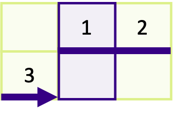
Sending sub-arrays of an array
By using a vector type, send the middle four elements (6, 7, 10, 11) in the following 4 x 4 matrix from rank 0 to rank 1,
int matrix[4][4] = {
  { 1,  2,  3,  4},
  { 5,  6,  7,  8},
  { 9, 10, 11, 12},
  {13, 14, 15, 16}
};
You can re-use most of your code from the previous exercise as your starting point, replacing the 2 x 3 matrix with the 4 x 4 matrix above and modifying the vector type and communication functions as required.
Solution
The receiving rank(s) should receive the numbers 6, 7, 10 and 11 if your solution is correct. In the solution below, we have created a vector with a count and block length of 2 and with a stride of 4. The first two arguments means two vectors of block length 2 will be sent. The stride of 4 results from that there are 4 elements between the start of each distinct block as shown in the image below,
You must always remember to send the address for the starting point of the first block as the send buffer, which is why
&array[1][1]is the first argument inMPI_Send().#include <mpi.h> #include <stdio.h> int main(int argc, char **argv) { int matrix[4][4] = { { 1, 2, 3, 4}, { 5, 6, 7, 8}, { 9, 10, 11, 12}, {13, 14, 15, 16} }; int my_rank; int num_ranks; MPI_Init(&argc, &argv); MPI_Comm_rank(MPI_COMM_WORLD, &my_rank); MPI_Comm_size(MPI_COMM_WORLD, &num_ranks); if (num_ranks != 2) { if (my_rank == 0) { printf("This example only works with 2 ranks\n"); } MPI_Abort(MPI_COMM_WORLD, 1); } MPI_Datatype sub_array_t; MPI_Type_vector(2, 2, 4, MPI_INT, &sub_array_t); MPI_Type_commit(&sub_array_t); if (my_rank == 0) { MPI_Send(&matrix[1][1], 1, sub_array_t, 1, 0, MPI_COMM_WORLD); } else { int buffer[4]; MPI_Status status; MPI_Recv(buffer, 4, MPI_INT, 0, 0, MPI_COMM_WORLD, &status); printf("Rank %d received the following:", my_rank); for (int i = 0; i < 4; ++i) { printf(" %d", buffer[i]); } printf("\n"); } MPI_Type_free(&sub_array_t); return MPI_Finalize(); }

Key Points
Any data being transferred should be a single contiguous block of memory
By defining derived data types, we can more easily send data which is not contiguous
Porting Serial Code to MPI
Overview
Teaching: 0 min
Exercises: 0 minQuestions
What is the best way to write a parallel code?
How do I parallelise my existing serial code?
Objectives
Identify which parts of a serial program would benefit from parallelisation
Explore how to convert a serial program into an MPI version
Differentiate between choices of communication pattern and algorithm design
Explain the importance of testing a parallel version against its serial version
In this section we will look at converting a complete code from serial to parallel in a number of steps.
An Example Iterative Poisson Solver
This episode is based on a code that solves the Poisson’s equation using an iterative method. Poisson’s equation appears in almost every field in physics, and is frequently used to model many physical phenomena such as heat conduction, and applications of this equation exist for both two and three dimensions. In this case, the equation is used in a simplified form to describe how heat diffuses in a one dimensional metal stick.
In the simulation the stick is split into a given number of slices, each with its own temperature.
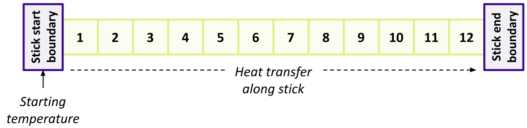
The temperature of the stick itself across each slice is initially set to zero, whilst at one boundary of the stick the amount of heat is set to 10. The code applies steps that simulates heat transfer along it, bringing each slice of the stick closer to a solution until it reaches a desired equilibrium in temperature along the whole stick.
Let’s download the code, which can be found here, and take a look at it now.
At a High Level - main()
We’ll begin by looking at the main() function at a high level.
#define MAX_ITERATIONS 25000
#define GRIDSIZE 12

...

int main(int argc, char **argv) {

  // The heat energy in each block
  float *u, *unew, *rho;
  float h, hsq;
  double unorm, residual;
  int i;

  u = malloc(sizeof(*u) * (GRIDSIZE+2));
  unew = malloc(sizeof(*unew) * (GRIDSIZE+2));
  rho = malloc(sizeof(*rho) * (GRIDSIZE+2));
It first defines two constants that govern the scale of the simulation:
MAX_ITERATIONS: determines the maximum number of iterative steps the code will attempt in order to find a solution with sufficiently low equilibriumGRIDSIZE: the number of slices within our stick that will be simulated. Increasing this will increase the number of stick slices to simulate, which increases the processing required
Next, it declares some arrays used during the iterative calculations:
u: each value represents the current temperature of a slice in the stickunew: during an iterative step, is used to hold the newly calculated temperature of a slice in the stickrho: holds a separate coefficient for each slice of the stick, used as part of the iterative calculation to represent potentially different boundary conditions for each stick slice. For simplicity, we’ll assume completely homogeneous boundary conditions, so these potentials are zero
Note we are defining each of our array sizes with two additional elements, the first of which represents a touching ‘boundary’ before the stick, i.e. something with a potentially different temperature touching the stick. The second added element is at the end of the stick, representing a similar boundary at the opposite end.
The next step is to initialise the initial conditions of the simulation:
  // Set up parameters
  h = 0.1;
  hsq = h * h;
  residual = 1e-5;

  // Initialise the u and rho field to 0
  for (i = 0; i <= GRIDSIZE + 1; ++i) {
    u[i] = 0.0;
    rho[i] = 0.0;
  }

  // Create a start configuration with the heat energy
  // u=10 at the x=0 boundary for rank 1
  u[0] = 10.0;
residual here refers to the threshold of temperature equilibrium along the stick we wish to achieve. Once it’s within this threshold, the simulation will end.
Note that initially, u is set entirely to zero, representing a temperature of zero along the length of the stick.
As noted, rho is set to zero here for simplicity.
Remember that additional first element of u? Here we set it to a temperature of 10.0 to represent something with that temperature touching the stick at one end, to initiate the process of heat transfer we wish to simulate.
Next, the code iteratively calls poisson_step() to calculate the next set of results, until either the maximum number of steps is reached, or a particular measure of the difference in temperature along the stick returned from this function (unorm) is below a particular threshold.
  // Run iterations until the field reaches an equilibrium
  // and no longer changes
  for (i = 0; i < NUM_ITERATIONS; ++i) {
    unorm = poisson_step(u, unew, rho, hsq, GRIDSIZE);
    if (sqrt(unorm) < sqrt(residual)) {
      break;
    }
  }
Finally, just for show, the code outputs a representation of the result - the end temperature of each slice of the stick.
  printf("Final result:\n");
  for (int j = 1; j <= GRIDSIZE; ++j) {
    printf("%d-", (int) u[j]);
  }
  printf("\n");
  printf("Run completed in %d iterations with residue %g\n", i, unorm);
}
The Iterative Function - poisson_step()
The poisson_step() progresses the simulation by a single step. After it accepts its arguments, for each slice in the stick it calculates a new value based on the temperatures of its neighbours:
  for (int i = 1; i <= points; ++i) {
     float difference = u[i-1] + u[i+1];
     unew[i] = 0.5 * (difference - hsq * rho[i]);
  }
Next, it calculates a value representing the overall cumulative change in temperature along the stick compared to its previous state, which as we saw before, is used to determine if we’ve reached a stable equilibrium and may exit the simulation:
  unorm = 0.0;
  for (int i = 1; i <= points; ++i) {
     float diff = unew[i] - u[i];
     unorm += diff * diff;
  }
And finally, the state of the stick is set to the newly calculated values, and unorm is returned from the function:
  // Overwrite u with the new field
  for (int i = 1 ;i <= points; ++i) {
     u[i] = unew[i];
  }

  return unorm;
}
Compiling and Running the Poisson Code
You may compile and run the code as follows:
gcc poisson.c -o poisson -lm
./poisson
And should see the following:
Final result:
9-8-7-6-6-5-4-3-3-2-1-0-
Run completed in 182 iterations with residue 9.60328e-06
Here, we can see a basic representation of the temperature of each slice of the stick at the end of the simulation, and how the initial 10.0 temperature applied at the beginning of the stick has transferred along it to this final state.
Ordinarily, we might output the full sequence to a file, but we’ve simplified it for convenience here.
Approaching Parallelism
So how should we make use of an MPI approach to parallelise this code? A good place to start is to consider the nature of the data within this computation, and what we need to achieve.
For a number of iterative steps, currently the code computes the next set of values for the entire stick.
So at a high level one approach using MPI would be to split this computation by dividing the stick into sections each with a number of slices, and have a separate rank responsible for computing iterations for those slices within its given section.
Essentially then, for simplicity we may consider each section a stick on its own, with either two neighbours at touching boundaries (for middle sections of the stick), or one touching boundary neighbour (for sections at the beginning and end of the stick, which also have either a start or end stick boundary touching them). For example, considering a GRIDSIZE of 12 and three ranks:
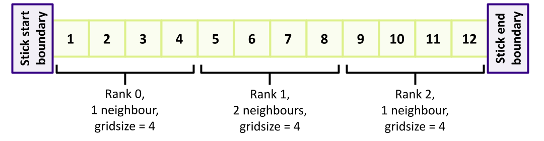
We might also consider subdividing the number of iterations, and parallelise across these instead. However, this is far less compelling since each step is completely dependent on the results of the prior step, so by its nature steps must be done serially.
The next step is to consider in more detail this approach to parallelism with our code.
Parallelism and Data Exchange
Looking at the code, which parts would benefit most from parallelisation, and are there any regions that require data exchange across its processes in order for the simulation to work as we intend?
Solution
Potentially, the following regions could be executed in parallel:
- The setup, when initialising the fields
- The calculation of each time step,
unew- this is the most computationally intensive of the loops- Calculation of the cumulative temperature difference,
unorm- Overwriting the field
uwith the result of the new calculationAs
GRIDSIZEis increased, these will take proportionally more time to complete, so may benefit from parallelisation.However, there are a few regions in the code that will require exchange of data across the parallel executions to work correctly:
- Calculation of
unormis a sum that requires difference data from all sections of the stick, so we’d need to somehow communicate these difference values to a single rank that computes and receives the overall sum- Each section of the stick does not compute a single step in isolation, it needs boundary data from neighbouring sections of the stick to arrive at its computed temperature value for that step, so we’d need to communicate temperature values between neighbours (i.e. using a nearest neighbours communication pattern)
We also need to identify any sizeable serial regions. The sum of the serial regions gives the minimum amount of time it will take to run the program. If the serial parts are a significant part of the algorithm, it may not be possible to write an efficient parallel version.
Serial Regions
Examine the code and try to identify any serial regions that can’t (or shouldn’t) be parallelised.
Solution
There aren’t any large or time consuming serial regions, which is good from a parallelism perspective. However, there are a couple of small regions that are not amenable to running in parallel:
- Setting the
10.0initial temperature condition at the stick ‘starting’ boundary. We only need to set this once at the beginning of the stick, and not at the boundary of every section of the stick- Printing a representation of the final result, since this only needs to be done once to represent the whole stick, and not for every section.
So we’d need to ensure only one rank deals with these, which in MPI is typically the zeroth rank. This also makes sense in terms of our parallelism approach, since the zeroth rank would be the beginning of the stick, where we’d set the initial boundary temperature.
Parallelising our Code
So now let’s apply what we’ve learned about MPI together with our consideration of the code.
First, make a copy of the poisson.c code that we will work on (don’t modify the original, we’ll need this later!).
In the shell, for example:
cp poisson.c poisson_mpi.c
And then we can add our MPI parallelisation modifications to poisson_mpi.c
We’ll start at a high level with main(), although first add #include <mpi.h> at the top of our code so we can make use of MPI.
We’ll do this parallelisation in a number of stages.
In MPI, all ranks execute the same code. When writing a parallel code with MPI, a good place to start is to think about a single rank. What does this rank need to do, and what information does it need to do it?
The first goal should be to write a simple code that works correctly. We can always optimise further later!
main(): Adding MPI at a High-level
Then as we usually do, let’s initialise MPI and obtain our rank and total number of ranks.
With the latter information, we can then calculate how many slices of the stick this rank will compute.
Near the top of main() add the following:
  int rank, n_ranks, rank_gridsize;

  MPI_Init(&argc, &argv);

  // Find the number of slices calculated by each rank
  // The simple calculation here assumes that GRIDSIZE is divisible by n_ranks
  MPI_Comm_rank(MPI_COMM_WORLD, &rank);
  MPI_Comm_size(MPI_COMM_WORLD, &n_ranks);
  rank_gridsize = GRIDSIZE / n_ranks;
Using rank_gridsize, we can now amend our initial array declaration sizes to use this instead:
  u = malloc(sizeof(*u) * (rank_gridsize + 2));
  unew = malloc(sizeof(*unew) * (rank_gridsize + 2));
  rho = malloc(sizeof(*rho) * (rank_gridsize + 2));
Then at the very end of main() let’s complete our use of MPI:
  MPI_Finalize();
}
main(): Initialising the Simulation and Printing the Result
Since we’re not initialising for the entire stick (GRIDSIZE) but just the section apportioned to our rank (rank_gridsize), we need to amend the loop that initialises u and rho accordingly, to:
  // Initialise the u and rho field to 0
  for (i = 0; i <= rank_gridsize + 1; ++i) {
    u[i] = 0.0;
    rho[i] = 0.0;
  }
As we found out in the Serial Regions exercise, we need to ensure that only a single rank (rank zero) needs to initiate the starting temperature within it’s section, so we need to put a condition on that initialisation:
  // Create a start configuration with the heat energy
  // u = 10 at the x = 0 boundary for rank 0
  if (rank == 0) {
    u[0] = 10.0;
  }
We also need to collect the overall results from all ranks and output that collected result, but again, only for rank zero.
To collect the results from all ranks (held in u) we can use MPI_Gather(), to send all u results to rank zero to hold in a results array.
Note that this will also include the result from rank zero!
Add the following to the list of declarations at the start of main():
float *resultbuf;
Then before MPI_Finalize() let’s amend the code to the following:
  // Gather results from all ranks
  // We need to send data starting from the second element of u, since u[0] is a boundary
  resultbuf = malloc(sizeof(*resultbuf) * GRIDSIZE);
  MPI_Gather(&u[1], rank_gridsize, MPI_FLOAT, resultbuf, rank_gridsize, MPI_FLOAT, 0, MPI_COMM_WORLD);

  if (rank == 0) {
    printf("Final result:\n");
    for (int j = 0; j < GRIDSIZE; j++) {
      printf("%d-", (int) resultbuf[j]);
    }
    printf("\nRun completed in %d iterations with residue %g\n", i, unorm);
  }
MPI_Gather() is ideally suited for our purposes, since results from ranks are arranged within resultbuf in rank order,
so we end up with all slices across all ranks representing the entire stick.
However, note that we need to send our data starting from u[1], since u[0] is the section’s boundary value we don’t want to include.
This has an interesting effect we need to account for - note the change to the for loop.
Since we are gathering data from each rank (including rank 0) starting from u[1], resultbuf will not contain any section boundary values so our loop no longer needs to skip the first value.
main(): Invoking the Step Function
Before we parallelise the poisson_step() function, let’s amend how we invoke it and pass it some additional parameters it will need.
We need to amend how many slices it will compute, and add the rank and n_ranks variables, since we know from Parallelism and Data Exchange that it will need to perform some data exchange with other ranks:
unorm = poisson_step(u, unew, rho, hsq, rank_gridsize, rank, n_ranks);
poisson_step(): Updating our Function Definition
Moving into the poisson_step() function, we first amend our function to include the changes to parameters:
double poisson_step(
  float *u, float *unew, float *rho,
  float hsq, int points,
  int rank, int n_ranks
) {
poisson_step(): Calculating a Global unorm
We know from Parallelism and Data Exchange that we need to calculate unorm across all ranks.
We already have it calculated for separate ranks, so need to reduce those values in an MPI sense to a single summed value.
For this, we can use MPI_Allreduce().
Insert the following into the poisson_step() function, putting the declarations at the top of the function,
and the MPI_Allreduce() after the calculation of unorm:
  double unorm, global_unorm;

  MPI_Allreduce(&unorm, &global_unorm, 1, MPI_DOUBLE, MPI_SUM, MPI_COMM_WORLD);
So here, we use this function in an MPI_SUM mode, which will sum all instances of unorm and place the result in a single (1) value global_unorm`.
We must also remember to amend the return value to this global version, since we need to calculate equilibrium across the entire stick:
  return global_unorm;
}
poisson_step(): Communicate Boundaries to Neighbours
In order for our parallel code to work, we know from Parallelism and Data Exchange that each section of slices is not computed in isolation.
After we’ve computed new values we need to send our boundary slice values to our neighbours if those neighbours exist -
the beginning and end of the stick will each only have one neighbour, so we need to account for that.
We also need to ensure that we don’t encounter a deadlock situation when exchanging the data between neighbours. They can’t all send to the rightmost neighbour simultaneously, since none will then be waiting and able to receive. We need a message exchange strategy here, so let’s have all odd-numbered ranks send their data first (to be received by even ranks), then have our even ranks send their data (to be received by odd ranks). Such an order might look like this (highlighting the odd ranks - only one in this example - with the order of communications indicated numerically):
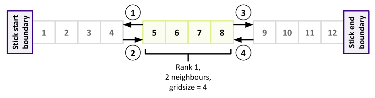
So following the MPI_Allreduce() we’ve just added, let’s deal with odd ranks first (again, put the declarations at the top of the function):
  float sendbuf, recvbuf;
  MPI_Status mpi_status;

  // The u field has been changed, communicate it to neighbours
  // With blocking communication, half the ranks should send first
  // and the other half should receive first
  if ((rank % 2) == 1) {
    // Ranks with odd number send first

    // Send data down from rank to rank - 1
    sendbuf = unew[1];
    MPI_Send(&sendbuf, 1, MPI_FLOAT, rank - 1, 1, MPI_COMM_WORLD);
    // Receive data from rank - 1
    MPI_Recv(&recvbuf, 1, MPI_FLOAT, rank - 1, 2, MPI_COMM_WORLD, &mpi_status);
    u[0] = recvbuf;

    if (rank != (n_ranks - 1)) {
      // Send data up to rank + 1 (if I'm not the last rank)
      MPI_Send(&u[points], 1, MPI_FLOAT, rank + 1, 1, MPI_COMM_WORLD);
      // Receive data from rank + 1
      MPI_Recv(&u[points + 1], 1, MPI_FLOAT, rank + 1, 2, MPI_COMM_WORLD, &mpi_status);
    }
Here we use C’s inbuilt modulus operator (%) to determine if the rank is odd.
If so, we exchange some data with the rank preceding us, and the one following.
We first send our newly computed leftmost value (at position 1 in our array) to the rank preceding us.
Since we’re an odd rank, we can always assume a rank preceding us exists,
since the earliest odd rank 1 will exchange with rank 0.
Then, we receive the rightmost boundary value from that rank.
Then, if the rank following us exists, we do the same, but this time we send the rightmost value at the end of our stick section, and receive the corresponding value from that rank.
These exchanges mean that - as an odd rank - we now have effectively exchanged the states of the start and end of our slices with our respective neighbours.
And now we need to do the same for those neighbours (the even ranks), mirroring the same communication pattern but in the opposite order of receive/send. From the perspective of evens, it should look like the following (highlighting the two even ranks):
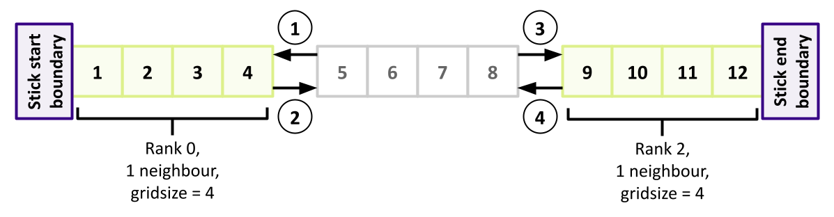
  } else {
    // Ranks with even number receive first

    if (rank != 0) {
      // Receive data from rank - 1 (if I'm not the first rank)
      MPI_Recv(&u[0], 1, MPI_FLOAT, rank - 1, 1, MPI_COMM_WORLD, &mpi_status);
      // Send data down to rank-1
      MPI_Send(&u[1], 1, MPI_FLOAT, rank - 1, 2, MPI_COMM_WORLD);
    }

    if (rank != (n_ranks - 1)) {
      // Receive data from rank + 1 (if I'm not the last rank)
      MPI_Recv(&u[points + 1], 1, MPI_FLOAT, rank + 1, 1, MPI_COMM_WORLD, &mpi_status);
      // Send data up to rank+1
      MPI_Send(&u[points], 1, MPI_FLOAT, rank + 1, 2, MPI_COMM_WORLD);
    }
  }
Once complete across all ranks, every rank will then have the slice boundary data from its neighbours ready for the next iteration.
Running our Parallel Code
You can obtain a full version of the parallelised Poisson code from here. Now we have the parallelised code in place, we can compile and run it, e.g.:
mpicc poisson_mpi.c -o poisson_mpi -lm
mpirun -n 2 poisson_mpi
Final result:
9-8-7-6-6-5-4-3-3-2-1-0-
Run completed in 182 iterations with residue 9.60328e-06
Note that as it stands, the implementation assumes that GRIDSIZE is divisible by n_ranks.
So to guarantee correct output, we should use only
Testing our Parallel Code
We should always ensure that as our parallel version is developed, that it behaves the same as our serial version. This may not be possible initially, particularly as large parts of the code need converting to use MPI, but where possible, we should continue to test. So we should test once we have an initial MPI version, and as our code develops, perhaps with new optimisations to improve performance, we should test then too.
An Initial Test
Test the mpi version of your code against the serial version, using 1, 2, 3, and 4 ranks with the MPI version. Are the results as you would expect? What happens if you test with 5 ranks, and why?
Solution
Using these ranks, the MPI results should be the same as our serial version. Using 5 ranks, our MPI version yields
9-8-7-6-5-4-3-2-1-0-0-0-which is incorrect. This is because therank_gridsize = GRIDSIZE / n_rankscalculation becomesrank_gridsize = 12 / 5, which produces 2.4. This is then converted to the integer 2, which means each of the 5 ranks is only operating on 2 slices each, for a total of 10 slices. This doesn’t fillresultbufwith results representing an expectedGRIDSIZEof 12, hence the incorrect answer.This highlights another aspect of complexity we need to take into account when writing such parallel implementations, where we must ensure a problem space is correctly subdivided. In this case, we could implement a more careful way to subdivide the slices across the ranks, with some ranks obtaining more slices to make up the shortfall correctly.
Limitations!
You may remember that for the purposes of this episode we’ve assumed a homogeneous stick, by setting the
rhocoefficient to zero for every slice. As a thought experiment, if we wanted to address this limitation and model an inhomogeneous stick with different static coefficients for each slice, how could we amend our code to allow this correctly for each slice across all ranks?Solution
One way would be to create a static lookup array with a
GRIDSIZEnumber of elements. This could be defined in a separate.hfile and imported using#include. Each rank could then read therhovalues for the specific slices in its section from the array and use those. At initialisation, instead of setting it to zero we could do:rho[i] = rho_coefficients[(rank * rank_gridsize) + i]
Key Points
Start from a working serial code
Write a parallel implementation for each function or parallel region
Connect the parallel regions with a minimal amount of communication
Continuously compare the developing parallel code with the working serial code
Optimising MPI Applications
Overview
Teaching: 0 min
Exercises: 0 minQuestions
How can we understand how well our code performs as resources increase?
Objectives
Describe and differentiate between strong and weak scaling
Test the strong and weak scaling performance of our MPI Poisson code
Use a profiler to identify performance characteristics of our MPI application
Now we have parallelised our code, we should determine how well it performs. Given the various ways code can be parallellised, the underlying scientific implementation, and the type and amount of data the code is expected to process, the performance of different parallelised code can vary hugely under different circumstances, particularly given different numbers of CPUs assigned to running the code in parallel. It’s a good idea to understand how the code will operate in a parallel sense, in order to make best (in particular, efficient) use of underlying HPC infrastructure. Also, we may want to consider how best to optimise the code to make more efficient use of its parallelisation.
Therefore, it’s really helpful to understand how well our code scales in performance terms as we increase the resources available to it.
Characterising the Scalability of Code
We first need a means to measure the performance increase of a particular program as we assign more processors to it, i.e. the speedup.
The speedup when running a parallel program on multiple processors can be defined as
[\mathrm{speedup} = t_1 / t_N]
Where:
- \(t_1\) is the computational time for running the software using one processor
- \(t_N\) is the computational time running the same software with N processors
Ideally, we would like software to have a linear speedup that is equal to the number of processors (speedup = N), as that would mean that every processor would be contributing 100% of its computational power. Unfortunately, this is a very challenging goal for real applications to attain, since there is always an overhead to making parallel use of greater resources. In addition, in a program there is always some portion of it which must be executed in serial (such as initialisation routines, I/O operations and inter-communication) which cannot be parallelised. This limits how much a program can be speeded up, as the program will always take at least the length of the serial portion.
Amdahl’s Law and Strong Scaling
There is a theoretical limit in what parallelization can achieve, and it is encapsulated in “Amdahl’s Law”:
[\mathrm{speedup} = 1 / (s + p / N)]
Where:
- \(s\) is the proportion of execution time spent on the serial part
- \(p\) is the proportion of execution time spent on the part that can be parallelized
- \(N\) is the number of processors
Amdahl’s law states that, for a fixed problem, the upper limit of speedup is determined by the serial fraction of the code - most real world applications have some serial portion or unintended delays (such as communication overheads) which will limit the code’s scalability. This is called strong scaling and its consequences can be understood from the figure below.
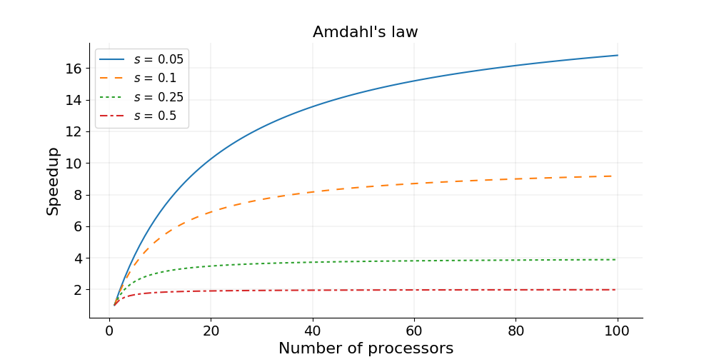
Amdahl’s Law in Practice
Consider a program that takes 20 hours to run using one core. If a particular part of the program, which takes one hour to execute, cannot be parallelized (s = 1/20 = 0.05), and if the code that takes up the remaining 19 hours of execution time can be parallelized (p = 1 − s = 0.95), then regardless of how many processors are devoted to a parallelized execution of this program, the minimum execution time cannot be less than that critical one hour. Hence, the theoretical speedup is limited to at most 20 times (when N = ∞, speedup = 1/s = 20).
Strong scaling is defined as how the solution time varies with the number of processors for a fixed total problem size. Linear strong scaling if the speedup (work units completed per unit time) is equal to the number of processing elements used. It’s harder to achieve good strong-scaling at larger process counts since communication overhead typically increases with the number of processes used.
Testing Code Performance on SLURM
We also need a way to test our code on our HPC infrastructure of choice. This will likely vary from system to system depending on your infrastructure configuration, but for the COSMA site on DiRAC this may look something like (replacing the
<account>,<queue>,<directory_containing_poisson_executable>accordingly):#!/usr/bin/env bash #SBATCH --account=<account> #SBATCH --partition=<queue> #SBATCH --job-name=mpi-poisson #SBATCH --time=00:05:00 #SBATCH --nodes=1 #SBATCH --ntasks=1 #SBATCH --mem=4M #SBATCH --chdir=<directory_containing_poisson_executable> module unload gnu_comp module load gnu_comp/11.1.0 module load openmpi/4.1.4 time mpirun -n 1 poisson_mpiSo here, after loading the required compiler and OpenMPI modules, we use the
timecommand to output how long the process took to run for a given number of processors. and ensure we specifyntaskscorrectly as the required number of cores we wish to use.We can then submit this using
sbatch, e.g.sbatch poisson-mpi.sh, with the output captured by default in aslurm-....outfile which will include the time taken to run the program.
Strong Scaling - How Does our Code Perform?
Strong scaling means increasing the number of ranks without changing the problem size. An algorithm with good strong scaling behaviour allows you to solve a problem more quickly by making use of more cores.
In
poisson_mpi.c, ensureMAX_ITERATIONSis set to25000andGRIDSIZEis512.Try submitting your program with an increasing number of ranks as we discussed earlier. What are the limitations on scaling?
Solution
Exact numbers depend on the machine you’re running on, but with a small number of ranks (up to 4) you should see the time decrease with the number of ranks. At around 5 ranks the result is a bit worse and doubling again to 16 has little effect.
The figure below shows an example of the scaling with
GRIDSIZE=512andGRIDSIZE=2048.
In the example, which runs on a machine with two 20-core Intel Xeon Scalable CPUs, using 32 ranks actually takes more time. The 32 ranks don’t fit on one CPU and communicating between the the two CPUs takes more time, even though they are in the same machine.
The communication could be made more efficient. We could use non-blocking communication and do some of the computation while communication is happening.
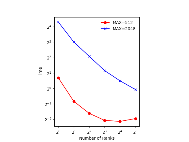
Gustafson’s Law and Weak Scaling
In practice the sizes of problems scale with the amount of available resources, and so we also need a measure for a relative speedup which takes into account increasing problem sizes.
Gustafson’s law is based on the approximations that the parallel part scales linearly with the amount of resources, and that the serial part does not increase with respect to the size of the problem. It provides a formula for scaled speedup:
[\mathrm{scaled\ speedup} = s + p × N]
where \(s\), \(p\) and \(N\) have the same meaning as in Amdahl’s law. With Gustafson’s law the scaled speedup increases linearly with respect to the number of processors (with a slope smaller than one), and there is no upper limit for the scaled speedup. This is called weak scaling, where the scaled speedup is calculated based on the amount of work done for a scaled problem size (in contrast to Amdahl’s law which focuses on fixed problem size).
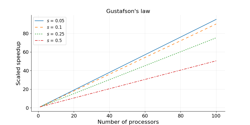
Weak scaling is defined as how the solution time varies with the number of processors for a fixed problem size per processor. If the run time stays constant while the workload is increased in direct proportion to the number of processors, then the solution is said to exhibit linear weak scaling.
Weak Scaling - How Does our Code Perform?
Weak scaling refers to increasing the size of the problem while increasing the number of ranks. This is much easier than strong scaling and there are several algorithms with good weak scaling. In fact our algorithm for integrating the Poisson equation might well have perfect weak scaling.
Good weak scaling allows you to solve much larger problems using HPC systems.
Run the Poisson solver with an increasing number of ranks, setting
GRIDSIZEto(n_ranks+1) * 128each time. Remember you’ll need to recompile the code each time before submitting it. How does it behave?Solution
Depending on the machine you’re running on, the runtime should be relatively constant. Runtime will increase if you need to use nodes that are further away from each other in the network.
The figure below shows an example of the scaling with
GRIDSIZE=128*n_ranks.
In this case all the ranks are running on the same node with 40 cores. The increase in runtime is probably due to the memory bandwidth of the node being used by a larger number of cores.
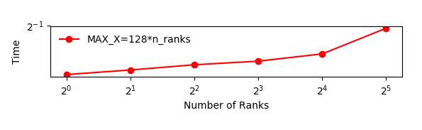
Other Factors Affecting Performance
Communication Speed and Latency
The other significant factors in the speed of a parallel program are communication speed and latency.
Communication speed is determined by the amount of data one needs to send/receive, and the bandwidth of the underlying hardware for the communication. Latency consists of the software latency (how long the operating system needs in order to prepare for a communication), and the hardware latency (how long the hardware takes to send/receive even a small bit of data).
For a fixed-size problem, the time spent in communication is not significant when the number of ranks is small and the execution of parallel regions gets faster with the number of ranks. But if we keep increasing the number of ranks, the time spent in communication grows when multiple cores are involved with communication.
Surface-to-Volume Ratio
In a parallel algorithm, the data which is handled by a core can be considered in two parts: the part the CPU needs that other cores control, and a part that the core controls itself and can compute. The whole data which a CPU or a core computes is the sum of the two. The data under the control of the other cores is called “surface” and the whole data is called “volume”.
The surface data requires communications. The more surface there is, the more communications among CPUs/cores is needed, and the longer the program will take to finish.
Due to Amdahl’s law, you want to minimize the number of communications for the same surface since each communication takes finite amount of time to prepare (latency). This suggests that the surface data be exchanged in one communication if possible, not small parts of the surface data exchanged in multiple communications. Of course, sequential consistency should be obeyed when the surface data is exchanged.
Profiling our Code
Now we have a better understanding of how our code scales with resources and problem size, we may want to consider how to optimise the code to perform better. But we should be careful!
“We should forget about small efficiencies, say about 97% of the time: premature optimization is the root of all evil.” – Donald Knuth
Essentially, before attempting to optimize your own code, you should profile it. Typically, most of the runtime is spent in a few functions/subroutines, so you should focus your optimization efforts on those parts of the code. The good news is that there are helpful tools known as profilers that can help us.
Profilers help you find out where a program is spending its time and pinpoint places where optimising it makes sense. Many different types of profiling tools exist, but for MPI application we need parallel profilers.
Some examples of parallel profilers are:
- Scalasca - a free and open source parallel profiler developed by three German research centers.
- TAU
- VAMPIR
- Paraver
In this lesson we will use a simple tool called ARM Performance Reports which gives us an overview of how much time is spent in compute, MPI calls and I/O. Performance Reports is part of the ARM Forge (formerly Allinea Forge) suite of tools for parallel applications and is developed by the semiconductor and software design company ARM.
The suite also comes with a debugger (ARM DDT) and a profiler (ARM MAP). ARM MAP is a more advanced tool which allows the user to see how much time each individual line of code takes, and why. ARM DDT supports a wide range of parallel architectures and models, including MPI, UPC, CUDA and OpenMP.
Version 19 and higher of ARM Forge supports Python, in addition to Fortran and C/C++. To see which versions are available, type:
module avail allinea
For more information on ARM Forge see the product website.
Performance Reports
Ordinarily when profiling our code using such a tool,
it is advisable to create a short version of your program, limiting the
runtime to a few seconds or minutes.
Fortunately that’s something we can readily configure with our poisson_mpi.c code.
For now, set MAX_ITERATIONS to 25000 and GRIDSIZE to 512.
We first load the module for Performance Reports. How you do this will vary site-to-site, but for COSMA on DiRAC we can do:
module load armforge/23.1.0
module load allinea/ddt/18.1.2
Next, we run the executable using Performance Reports to analyse the program execution. Create a new version of our SLURM submission script we used before, which includes the following at the bottom of the script instead:
module load armforge/23.1.0
module load allinea/ddt/18.1.2

module unload gnu_comp
module load gnu_comp/11.1.0
module load openmpi/4.1.4

perf-report mpirun -n 4 poisson_mpi
And then submit it, e.g. sbatch perf-poisson-mpi.sh.
This creates two files, one .txt file which can be viewed in the
terminal and one .html file which can be opened in a browser
(you will need to scp the HTML file to your local machine to view it).
cat poisson_mpi_4p_1n_2024-01-30_15-38.txt
Command:        mpirun -n 4 poisson_mpi
Resources:      1 node (28 physical, 56 logical cores per node)
Memory:         503 GiB per node
Tasks:          4 processes
Machine:        <specific_node_displayed_here>
Architecture:   x86_64
CPU Family:     skylake-x
Start time:     Tue Jan 30 15:38:06 2024
Total time:     1 second
Full path:      <run_directory_displayed_here>

Summary: poisson_mpi is MPI-bound in this configuration
Compute:                                      6.6%     (0.0s) ||
MPI:                                         93.4%     (0.2s) |========|
I/O:                                          0.0%     (0.0s) |
This application run was MPI-bound (based on main thread activity). A breakdown of this time and advice for investigating further is in the MPI section below.

...
The graphical HTML output looks like this:
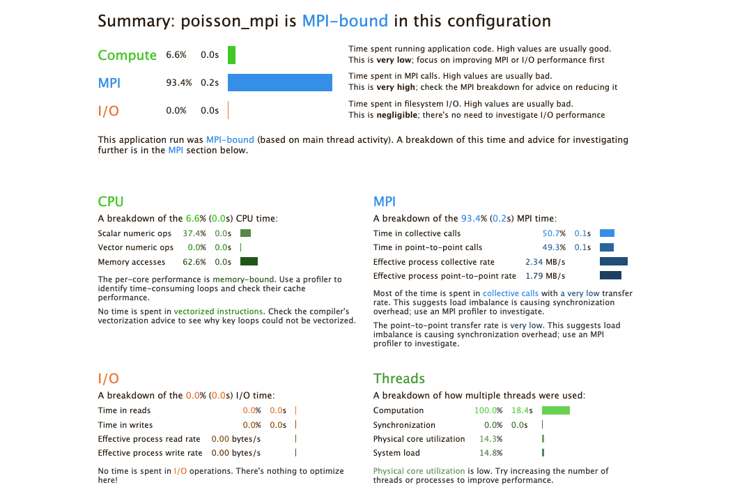
The output shows that when run in this way, the application is MPI bound, i.e. most time is spent in MPI communication. This typically means that the application does not scale well to the given number of processes. Either the number of processes should be decreased, or the problem size increased so that more time is spent in the actual compute sections of the code.
Profile Your Poisson Code
Compile, run and analyse your own MPI version of the poisson code.
How closely does it match the performance above? What are the main differences? Try reducing the number of processes used, rerun and investigate the profile. Is it still MPI-bound?
Increase the problem size, recompile, rerun and investigate the profile. What has changed now?
Iterative Improvement
In the Poisson code, try changing the location of the calls to
MPI_Send(). How does this affect performance?
A General Optimisation Workflow?
A general workflow for optimising a code, whether parallel or serial, is as follows:
- Profile
- Optimise
- Test correctness
- Measure efficiency
Then we can repeat this process as needed. But note that eventually this process will yield diminishing returns, and over-optimisation is a trap to avoid - hence the importance of continuing to measure efficiency as you progress.
Key Points
We can use Amdahl’s Law to identify the theoretical limit in what parallelisation can achieve for performance
Strong scaling is defined as how the solution time varies with the number of processors for a fixed total problem size
We can use Gustafson’s Law to calculate relative speedup which takes into account increasing problem sizes
Weak scaling is defined as how the solution time varies with the number of processors for a fixed problem size per processor
Use a profiler to profile code to understand its performance issues before optimising it
Ensure code is tested after optimisation to ensure its functional behaviour is still correct
Common Communication Patterns [Optional]
Overview
Teaching: 20 min
Exercises: 30 minQuestions
What are some common data communication patterns in MPI?
Objectives
Describe an example of how scatter and gather communication is used in mathematical matrix processing
Describe an example use of reduction within a Monte Carlo application
Describe how a spatial problem space can be decomposed into sub-domains for processing
Describe the features of halo exchange and how it applies to sub-domain processing
We have now come across the basic building blocks we need to create an MPI application. The previous episodes have covered how to split tasks between ranks to parallelise the workload, and how to communicate data between ranks; either between two ranks (point-to-point) or multiple at once (collective). The next step is to build upon these basic blocks, and to think about how we should structure our communication. The parallelisation and communication strategy we choose will depend on the underlying problem and algorithm. For example, a grid based simulation (such as in computational fluid dynamics) will need to structure its communication differently to a simulation which does not discretise calculations onto a grid of points. In this episode, we will look at some of the most common communication patterns.
Scatter and gather
Using the scatter and gather collective communication functions, to distribute work and bring the results back together, is a common pattern and finds a wide range of applications. To recap: in scatter communication, the root rank splits a piece of data into equal chunks and sends a chunk to each of the other ranks, as shown in the diagram below.
In gather communication all ranks send data to the root rank which combines them into a single buffer.
Scatter communication is useful for most algorithms and data access patterns, as is gather communication. At least for scattering, this communication pattern is generally easy to implement especially for embarrassingly parallel problems where the data sent to each rank is independent. Gathering data is useful for bringing results to a root rank to process further or to write to disk, and is also helpful for bring data together to generate diagnostic output.
Since scatter and gather communications are collective, the communication time required for this pattern increases as
the number of ranks increases. The amount of messages that needs to be sent increases logarithmically with the number of
ranks. The most efficient implementation of scatter and gather communication are to use the collective functions
(MPI_Scatter() and MPI_Gather()) in the MPI library.
One method for parallelising matrix multiplication is with a scatter and gather communication. To multiply two matrices, we follow the following equation,
[\left[ \begin{array}{cc} A_{11} & A_{12} \ A_{21} & A_{22}\end{array} \right] \cdot \left[ \begin{array}{cc}B_{11} & B_{12} \ B_{21} & B_{22}\end{array} \right] = \left[ \begin{array}{cc}A_{11} \cdot B_{11} + A_{12} \cdot B_{21} & A_{11} \cdot B_{12} + A_{12} \cdot B_{22} \ A_{21} \cdot B_{11} + A_{22} \cdot B_{21} & A_{21} \cdot B_{12}
- A_{22} \cdot B_{22}\end{array} \right]]
Each element of the resulting matrix is a dot product between a row in the first matrix (matrix A) and a column in the second matrix (matrix B). Each row in the resulting matrix depends on a single row in matrix A, and each column in matrix B. To split the calculation across ranks, one approach would be to scatter rows from matrix A and calculate the result for that scattered data and to combine the results from each rank to get the full result.
// Determine how many rows each matrix will compute and allocate space for a receive buffer
// receive scattered subsets from root rank. We'll use 1D arrays to store the matrices, as it
// makes life easier when using scatter and gather
int rows_per_rank = num_rows_a / num_ranks;
double *rank_matrix_a = malloc(rows_per_rank * num_rows_a * sizeof(double));
double *rank_matrix_result = malloc(rows_per_rank * num_cols_b * sizeof(double));

// Scatter matrix_a across ranks into rank_matrix_a. Each rank will compute a subset of
//  the result for the rows in rank_matrix_a
MPI_Scatter(matrix_a, rows_per_rank * num_cols_a, MPI_DOUBLE, rank_matrix_a, rows_per_rank * num_cols_a,
            MPI_DOUBLE, ROOT_RANK, MPI_COMM_WORLD);

// Broadcast matrix_b to all ranks, because matrix_b was only created on the root rank
// and each sub-calculation needs to know all elements in matrix_b
MPI_Bcast(matrix_b, num_rows_b * num_cols_b, MPI_DOUBLE, ROOT_RANK, MPI_COMM_WORLD);

// Function to compute result for the subset of rows of matrix_a
multiply_matrices(rank_matrix_a, matrix_b, rank_matrix_result);

// Use gather communication to get each rank's result for rank_matrix_a * matrix_b into receive
// buffer `matrix_result`. Our life is made easier since rank_matrix and matrix_result are flat (and contiguous)
// arrays, so we don't need to worry about memory layout
MPI_Gather(rank_matrix_result, rows_per_rank * num_cols_b, MPI_DOUBLE, matrix_result, rows_per_rank * num_cols_b,
           MPI_DOUBLE, ROOT_RANK, MPI_COMM_WORLD);
Reduction
A reduction operation is one that reduces multiple pieces of data into a single value, such as by summing values or finding the largest value in a collection of values. The use case for reductions throughout scientific code is wide, which makes it a very common communication pattern. Since reductions are a collective operation, the communication overheads increases with the number of ranks. It is again, like with scattering and gathering, best to use the reduction functions within the MPI library, rather than implementing the pattern ourselves.
Given the fact that reductions fit in almost any algorithm or data access pattern, there are countless examples to show a reduction communication pattern. In the next code example, a Monte Carlo algorithm is implemented which estimates the value of $\pi$. To do that, a billion random points are generated and checked whether they fall within or outside of a circle. The ratio of points in and outside of the circle is propotional to the value of $\pi$.
Since each point generated and its position within the circle is completely independent to the other points, the communication pattern is simple (this is also an example of an embarrassingly parallel problem) as we only need one reduction. To parallelise the problem, each rank generates a sub-set of the total number of points and a reduction is done at the end, to calculate the total number of points within the circle from the entire sample.
// 1 billion points is a lot, so we should parallelise this calculation
int total_num_points = (int)1e9;

// Each rank will check an equal number of points, with their own
// counter to track the number of points falling within the circle
int points_per_rank = total_num_points / num_ranks;
int rank_points_in_circle = 0;

// Seed each rank's RNG with a unique seed, otherwise each rank will have an
// identical result and it would be the same as using `points_per_rank` in total
// rather than `total_num_points`
srand(time(NULL) + my_rank);

// Generate a random x and y coordinate (between 0 - 1) and check to see if that
// point lies within the unit circle
for (int i = 0; i < points_per_rank; ++i) {
    double x = (double)rand() / RAND_MAX;
    double y = (double)rand() / RAND_MAX;
    if ((x * x) + (y * y) <= 1.0) {
        rank_points_in_circle++;  // It's in the circle, so increment the counter
    }
}

// Perform a reduction to sum up `rank_points_in_circle` across all ranks, this
// will be the total number of points in a circle for `total_num_point` iterations
int total_points_in_circle;
MPI_Reduce(&rank_points_in_circle, &total_points_in_circle, 1, MPI_INT, MPI_SUM, ROOT_RANK, MPI_COMM_WORLD);

//The estimate for π is proportional to the ratio of the points in the circle and the number of
// points generated
if (my_rank == ROOT_RANK) {
    double pi = 4.0 * total_points_in_circle / total_num_points;
    printf("Estimated value of π = %f\n", pi);
}
More reduction examples
Reduction operations are not only used in embarrassingly parallel Monte Carlo problems. Can you think of any other examples, or algorithms, where you might use a reduction pattern?
Solution
Here is a (non-exhaustive) list of examples where reduction operations are useful.
- Finding the maximum/minimum or average temperature in a simulation grid: by conducting a reduction across all the grid cells (which may have, for example, been scattered across ranks), you can easily find the maximum/minimum temperature in the grid, or sum up the temperatures to calculate the average temperature.
- Combining results into a global state: in some simulations, such as climate modelling, the simulation is split into discrete time steps. At the end of each time step, a reduction can be used to update the global state or combine together pieces of data (similar to a gather operation).
- Large statistical models: in a large statistical model, the large amounts of data can be processed by splitting it across ranks and calculating statistical values for the sub-set of data. The final values are then calculated by using a reduction operation and re-normalizing the values appropriately.
- Numerical integration: each rank will compute the area under the curve for its portion of the curve. The value of the integral for the entire curve is then calculated using a reduction operation.
Domain decomposition and halo exchange
If a problem depends on a (usually spatially) discretised grid, array of values or grid structure, such as in, for example, image processing, computational fluid dynamics, molecular dynamics or finite element analysis, then we can parallelise the tasks by splitting the problem into smaller sub-domains for each rank to work with. This is shown in the diagram below, where an image has been split into four smaller images which will be sent to a rank.

In most cases, these problems are usually not embarrassingly parallel, since additional communication is often required as the work is not independent and depends on data in other ranks, such as the value of neighbouring grid points or results from a previous iteration. As an example, in a molecular dynamics simulation, updating the state of a molecule depends on the state and interactions between other molecules which may be in another domain in a different rank.
A common feature of a domain decomposed algorithm is that communications are limited to a small number of other ranks that work on a sub-domain a short distance away. In such a case, each rank only needs a thin slice of data from its neighbouring rank(s) and send the same slice of its own data to the neighbour(s). The data received from neighbours forms a “halo” around the ranks own data, and shown in the next diagram, and is known as halo exchange.
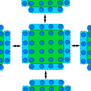
The matrix example from earlier is actually an example of domain decomposition, albeit a simple case, as the rows of the matrix were split across ranks. It’s a simple example, as additional data didn’t need to be communicated between ranks to solve the problem. There is, unfortunately, no best way or “one size fits all” type of domain decomposition, as it depends on the algorithm and data access required.
Domain decomposition
If we take image processing as an example, we can split the image like in the matrix example, where each rank gets some number of rows of the image to process. In this case, the code to scatter the rows of image is more or less identical to the matrix case from earlier. Another approach would be to decompose the image into smaller rectangles like in the image above. This is sometimes a better approach, as it allows for more efficient and balanced resource allocation and halo communication, but this is usually as the expense of increased memory usage and code complexity.
An example of 2D domain decomposition is shown in the next example, which uses a derived type (from the previous episode) to discretise the image into smaller rectangles and to scatter the smaller sub-domains to the other ranks.
// We have to first calculate the size of each rectangular region. In this example, we have
// assumed that the dimensions are perfectly divisible. We can determine the dimensions for the
// decomposition by using MPI_Dims_create()
int rank_dims[2] = { 0, 0 };
MPI_Dims_create(num_ranks, 2, rank_dims);
int num_rows_per_rank = num_rows / rank_dims[0];
int num_cols_per_rank = num_cols / rank_dims[1];
int num_elements_per_rank = num_rows_per_rank * num_cols_per_rank;

// The rectangular blocks we create are not contiguous in memory, so we have to use a
// derived data type for communication
MPI_Datatype sub_array_t;
int count = num_rows_per_rank;
int blocklength = num_cols_per_rank;
int stride = num_cols;
MPI_Type_vector(count, blocklength, stride, MPI_DOUBLE, &sub_array_t);
MPI_Type_commit(&sub_array_t);

// MPI_Scatter (and similar collective functions) do not work well with this sort of
// topology, so we unfortunately have to scatter the array manually
double *rank_image = malloc(num_elements_per_rank * sizeof(double));
scatter_sub_arrays_to_other_ranks(image, rank_image, sub_array_t, rank_dims, my_rank, num_rows_per_rank,
                                  num_cols_per_rank, num_elements_per_rank, num_cols);
Extra: Scattering the image to other ranks
As mentioned in the previous code example, distributing the 2D sub-domains across ranks doesn’t play well with collective functions. Therefore, we have to transfer the data manually using point-to-point communication. An example of how can be done is shown below.
// Function to convert row and col coordinates into an index for a 1d array
int index_into_2d(int row, int col, int num_cols) { return row * num_cols + col; }

// Fairly complex function to send sub-arrays of `image` to the other ranks
void scatter_sub_arrays_to_other_ranks(double *image, double *rank_image, MPI_Datatype sub_array_t, int rank_dims[2],
                                       int my_rank, int num_cols_per_rank, int num_rows_per_rank,
                                       int num_elements_per_rank, int num_cols)
{
   if (my_rank == ROOT_RANK) {
      int dest_rank = 0;
      for (int i = 0; i < rank_dims[0]) {
         for (int j = 0; j < rank_dims[1]) {
            // Send sub array to a non-root rank
            if(dest_rank != ROOT_RANK) {
               MPI_Send(&image[index_into_2d(num_rows_per_rank * i, num_cols_per_rank * j, num_cols)], 1, sub_array_t,
                        dest_rank, 0, MPI_COMM_WORLD);
            // Copy into root rank's rank image buffer
            } else {
              for (int ii = 0; ii < num_rows_per_rank; ++ii) {
                  for (int jj = 0; jj < num_cols_per_rank; ++jj) {
                     rank_image[index_into_2d(ii, jj, num_cols_per_rank)] = image[index_into_2d(ii, jj, num_cols)];
                  }
               }
            }
            dest_rank += 1;
         }
      }
   } else {
      MPI_Recv(rank_image, num_elements_per_rank, MPI_DOUBLE, ROOT_RANK, MPI_COMM_WORLD, MPI_STATUS_IGNORE);
   }
}
The function MPI_Dims_create() is a useful utility
function in MPI which is used to determine the dimensions of a Cartesian grid of ranks. In the above example, it’s
used to determine the number of rows and columns in each sub-array, given the number of ranks in the row and column
directions of the grid of ranks from MPI_Dims_create(). In addition to the code above, you may also want to create a
virtual Cartesian communicator topology to
reflect the decomposed geometry in the communicator as well, as this give access to a number of other utility functions
which makes communicating data easier.
Halo exchange
In domain decomposition methods, a “halo” refers to a region around the boundary of a sub-domain which contains a copy of the data from neighbouring sub-domains, which needed to perform computations that involve data from adjacent sub-domains. The halo region allows neighbouring sub-domains to share the required data efficiently, without the need for more than necessary communication.
In a grid-based domain decomposition, as in the image processing example, a halo is often one, or more, rows of pixels (or grid cells more generally) that surround a sub-domain’s “internal” cells. This is shown in the diagram below. In the diagram, the image has decomposed across two ranks in one direction (1D decomposition). Each blue region represents the halo for that rank, which has come from the region the respective arrow is point from.
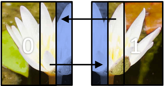
Halos, naturally, increase the memory overhead of the parallelisation as you need to allocate additional space in the
array or data structures to account for the halo pixels/cells. For example, in the above diagram, if the image was
discretised into more sub-domains so there are halos on both the left and right side of the sub-domain. In image
processing, a single strip of pixels is usually enough. If num_rows and num_cols are the number of rows of pixels
containing that many columns of pixels, then each sub-domain has dimensions num_rows and num_cols + 2. If the
decomposition was in two dimensions, then it would be num_rows + 2 and num_cols + 2. In other data structures like
graphs or unstructured grids, the halo will be an elements or nodes surrounding the sub-domain.
The example code below shows one method of communicating halo data between neighbouring ranks in a decomposition like in
the diagram above. The image has been decomposed into strips, which each rank working on a sub-image with dimensions
num_rows / num_ranks rows and num_cols columns. In the example,
MPI_Sendrecv() is used to send and receiving data
between neighbouring ranks.
Chain communication with
MPI_Sendrecv()
MPI_Sendrecv()combines both sending and receiving data in a single call. It allows a rank to send data to another rank, whilst receiving data from another. With this function we can usually set up a “chain” communication pattern, where each rank sends data to one neighbour and receives data from its other date, as shown in the diagram below.
In 1D domain decomposition, this is a helpful function to use as each rank will only want data from its neighbours.
int MPI_Sendrecv(
   void *sendbuf,
   int sendcount,
   MPI_Datatype sendtype,
   int dest,
   int sendtag,
   void *recvbuf,
   int recvcount,
   MPI_Datatype recvtype,
   int source,
   int recvtag,
   MPI_Comm comm,
   MPI_Status *status
);
*sendbuf:The data to be sent to destsendcount:The number of elements of data to be sent to destsendtype:The data type of the data to be sent to destdest:The rank where data is being sent to sendtag:The communication tag for the send *recvbuf:A buffer for data being received recvcount:The number of elements of data to receive recvtype:The data type of the data being received source:The rank where data is coming from recvtag:The communication tag for the receive comm:The communicator *status:The status handle for the receive
// Function to convert row and col coordinates into an index for a 1d array
int index_into_2d(int row, int col, int num_cols) { return row * num_cols + col; }

// `rank_image` is actually a little bigger, as we need two extra rows for a halo region for the top
//  and bottom of the row sub-domain
double *rank_image = malloc((num_rows + 2) * num_cols * sizeof(double));

// MPI_Sendrecv is designed for "chain" communications, so we need to figure out the next
// and previous rank. We use `MPI_PROC_NULL` (a special constant) to tell MPI that we don't
// have a partner to communicate to/receive from
int prev_rank = my_rank - 1 < 0 ? MPI_PROC_NULL : my_rank - 1;
int next_rank = my_rank + 1 > num_ranks - 1 ? MPI_PROC_NULL : my_rank + 1;

// Send the top row of the image to the bottom row of the previous rank, and receive
// the top row from the next rank
MPI_Sendrecv(&rank_image[index_into_2d(0, 1, num_cols)], num_rows, MPI_DOUBLE, prev_rank, 0,
             &rank_image[index_into_2d(num_rows - 1, 1, num_cols)], num_rows, MPI_DOUBLE, next_rank, 0,
             MPI_COMM_WORLD, MPI_STATUS_IGNORE);

// Send the bottom row into top row of the next rank, and the reverse from the previous rank
MPI_Sendrecv(&rank_image[index_into_2d(num_rows - 2, 1, num_cols)], num_rows, MPI_DOUBLE, next_rank, 0,
             &rank_image[index_into_2d(0, 1, num_cols)], num_rows, MPI_DOUBLE, prev_rank, 0, MPI_COMM_WORLD,
             MPI_STATUS_IGNORE);
Halo exchange in two dimensions
The previous code example shows one implementation of halo exchange in one dimension. Following from the code example showing domain decomposition in two dimensions, write down the steps (or some pseudocode) for the implementation of domain decomposition and halo exchange in two dimensions.
Solution
Communicating halos in a 2D domain decomposition is similar to the code example above, but we have two additional communications as we have to communicate four rows/columns of data: the top and bottom rows, and the left-most and right-most column of pixels. This is all easier said than done, though. The image below, that we’ve already seen, shows a depiction of halo exchange in 2D, where each sub-domain has a neighbour above and below and to the left and right of it.
To communicate the halos, we need to:
- Create a derived type to send a column of data for the correct number of rows of pixels. The top and bottom rows can be communicated without using a derived type, because the elements in a row are contiguous.
- For each sub-domain, we need to determine the neighbouring ranks, so we know which rank to send data to and which ranks to receive data from.
- Using the derived types and neighbouring ranks, communicate the top row of the sub-domain to the bottom halo row of the neighbouring top domain. We also need to repeat the same process for the bottom row to the neighbouring sub-domain below and so on for the left and right columns of halo data.
To re-build the sub-domains into one domain, we can do the reverse of the hidden code exert of the function
scatter_sub_arrays_to_other ranks. Instead of the root rank sending data, it instead receives data from the other ranks using the samesub_array_tderived type.
Key Points
There are many ways to communicate data, which we need to think about carefully
It’s better to use collective operations, rather than implementing similar behaviour yourself
Advanced Data Communication [Optional]
Overview
Teaching: 25 min
Exercises: 20 minQuestions
How do I communicate structures?
How do I communicate non-contiguous data which isn’t easy to express as a derived data type?
Objectives
Define and use an MPI structure to represent complex data
Use MPI to package non-contiguous data for communication
Use MPI to unpackage data into non-contiguous structures
In an earlier episode, we introduced the concept of derived data types to send vectors or a sub-array of a larger array,
which may or may not be contiguous in memory. Other than vectors, there are multiple other types of derived data types
that allow us to handle other complex data structures efficiently. In this episode, we will see how to create structure
derived types. Additionally, we will also learn how to use MPI_Pack() and MPI_Unpack() to manually pack complex data
structures and heterogeneous into a single contiguous buffer, when other methods of communication are too complicated or
inefficient.
Structures in MPI
Structures, commonly known as structs, are custom datatypes which contain multiple variables of (usually) different types. Some common use cases of structs, in scientific code, include grouping together constants or global variables, or they are used to represent a physical thing, such as a particle, or something more abstract like a cell on a simulation grid. When we use structs, we can write clearer, more concise and better structured code.
To communicate a struct, we need to define a derived datatype which tells MPI about the layout of the struct in memory.
Instead of MPI_Type_create_vector(), for a struct, we use,
MPI_Type_create_struct(),
int MPI_Type_create_struct(
   int count,
   int *array_of_blocklengths,
   MPI_Aint *array_of_displacements,
   MPI_Datatype *array_of_types,
   MPI_Datatype *newtype,
);
count: |
The number of fields in the struct |
*array_of_blocklengths: |
The length of each field, as you would use to send that field using MPI_Send() |
*array_of_displacements: |
The relative positions of each field in bytes |
*array_of_types: |
The MPI type of each field |
*newtype: |
The newly created data type for the struct |
The main difference between vector and struct derived types is that the arguments for structs expect arrays, since
structs are made up of multiple variables. Most of these arguments are straightforward, given what we’ve just seen for
defining vectors. But array_of_displacements is new and unique.
When a struct is created, it occupies a single contiguous block of memory. But there is a catch. For performance reasons, compilers insert arbitrary “padding” between each member for performance reasons. This padding, known as data structure alignment, optimises both the layout of the memory and the access of it. As a result, the memory layout of a struct may look like this instead:
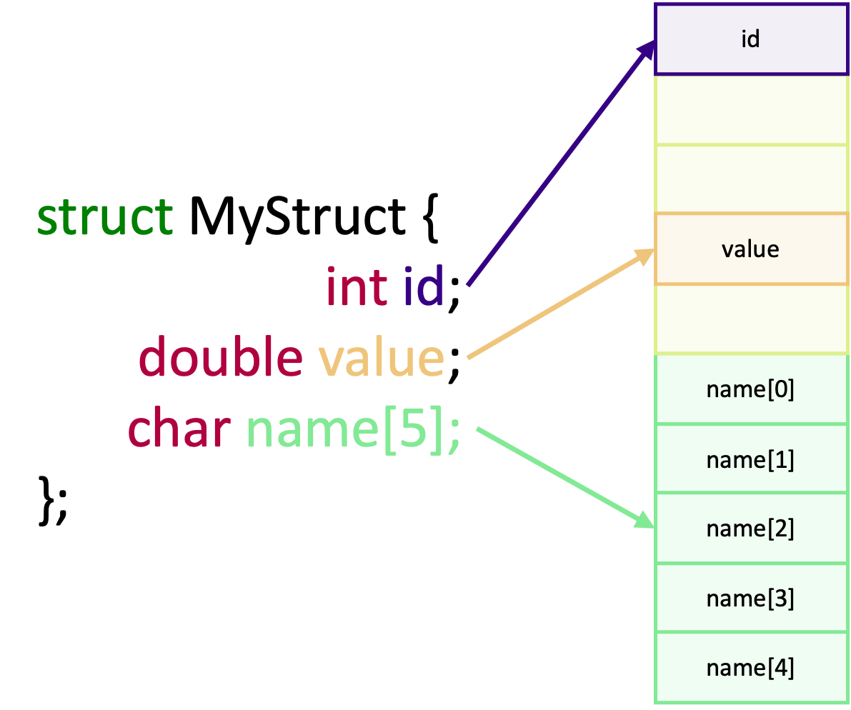
Although the memory used for padding and the struct’s data exists in a contiguous block, the actual data we care about
is not contiguous any more. This is why we need the array_of_displacements argument, which specifies the distance, in
bytes, between each struct member relative to the start of the struct. In practise, it serves a similar purpose of the
stride in vectors.
To calculate the byte displacement for each member, we need to know where in memory each member of a struct exists. To
do this, we can use the function MPI_Get_address(),
int MPI_Get_address{
   const void *location,
   MPI_Aint *address,
};
*location: |
A pointer to the variable we want the address of |
*address: |
The address of the variable, as an MPI_Aint (address integer) |
In the following example, we use MPI_Type_create_struct() and MPI_Get_address() to create a derived type for a
struct with two members,
// Define and initialize a struct, named foo, with an int and a double
struct MyStruct {
   int id;
   double value;
} foo = {.id = 0, .value = 3.1459};

// Create arrays to describe the length of each member and their type
int count = 2;
int block_lengths[2] = {1, 1};
MPI_Datatype block_types[2] = {MPI_INT, MPI_DOUBLE};

// Now we calculate the displacement of each member, which are stored in an
// MPI_Aint designed for storing memory addresses
MPI_Aint base_address;
MPI_Aint block_offsets[2];

MPI_Get_address(&foo, &base_address);            // First of all, we find the address of the start of the struct
MPI_Get_address(&foo.id, &block_offsets[0]);     // Now the address of the first member "id"
MPI_Get_address(&foo.value, &block_offsets[1]);  // And the second member "value"

// Calculate the offsets, by subtracting the address of each field from the
// base address of the struct
for (int i = 0; i < 2; ++i) {
   // MPI_Aint_diff is a macro to calculate the difference between two
   // MPI_Aints and is a replacement for:
   //       (MPI_Aint) ((char *) block_offsets[i] - (char *) base_address)
   block_offsets[i] = MPI_Aint_diff(block_offsets[i], base_address);
}

// We finally can create out struct data type
MPI_Datatype struct_type;
MPI_Type_create_struct(count, block_lengths, block_offsets, block_types, &struct_type);
MPI_Type_commit(&struct_type);

// Another difference between vector and struct derived types is that in
// MPI_Recv, we use the struct type. We have to do this because we aren't
// receiving a contiguous block of a single type of date. By using the type, we
// tell MPI_Recv how to understand the mix of data types and padding and how to
// assign those back to recv_struct
if (my_rank == 0) {
   MPI_Send(&foo, 1, struct_type, 1, 0, MPI_COMM_WORLD);
} else {
   struct MyStruct recv_struct;
   MPI_Recv(&recv_struct, 1, struct_type, 0, 0, MPI_COMM_WORLD, MPI_STATUS_IGNORE);
}

// Remember to free the derived type
MPI_Type_free(&struct_type);
Sending a struct
By using a derived data type, write a program to send the following struct
struct Node nodefrom one rank to another,struct Node { int id; char name[16]; double temperature; }; struct Node node = { .id = 0, .name = "Dale Cooper", .temperature = 42};You may wish to use this skeleton code as your stating point.
Solution
Your solution should look something like the code block below. When sending a static array (
name[16]), we have to use a count of 16 in theblock_lengthsarray for that member.#include <mpi.h> #include <stdio.h> struct Node { int id; char name[16]; double temperature; }; int main(int argc, char **argv) { int my_rank; int num_ranks; MPI_Init(&argc, &argv); MPI_Comm_rank(MPI_COMM_WORLD, &my_rank); MPI_Comm_size(MPI_COMM_WORLD, &num_ranks); if (num_ranks != 2) { if (my_rank == 0) { printf("This example only works with 2 ranks\n"); } MPI_Abort(MPI_COMM_WORLD, 1); } struct Node node = {.id = 0, .name = "Dale Cooper", .temperature = 42}; int block_lengths[3] = {1, 16, 1}; MPI_Datatype block_types[3] = {MPI_INT, MPI_CHAR, MPI_DOUBLE}; MPI_Aint base_address; MPI_Aint block_offsets[3]; MPI_Get_address(&node, &base_address); MPI_Get_address(&node.id, &block_offsets[0]); MPI_Get_address(&node.name, &block_offsets[1]); MPI_Get_address(&node.temperature, &block_offsets[2]); for (int i = 0; i < 3; ++i) { block_offsets[i] = MPI_Aint_diff(block_offsets[i], base_address); } MPI_Datatype node_struct; MPI_Type_create_struct(3, block_lengths, block_offsets, block_types, &node_struct); MPI_Type_commit(&node_struct); if (my_rank == 0) { MPI_Send(&node, 1, node_struct, 1, 0, MPI_COMM_WORLD); } else { struct Node recv_node; MPI_Recv(&recv_node, 1, node_struct, 0, 0, MPI_COMM_WORLD, MPI_STATUS_IGNORE); printf("Received node: id = %d name = %s temperature %f\n", recv_node.id, recv_node.name, recv_node.temperature); } MPI_Type_free(&node_struct); return MPI_Finalize(); }
What if I have a pointer in my struct?
Suppose we have the following struct with a pointer named
positionand some other fields,struct Grid { double *position; int num_cells; }; grid.position = malloc(3 * sizeof(double));If we use
malloc()to allocate memory forposition, how would we send data in the struct and the memory we allocated one rank to another? If you are unsure, try writing a short program to create a derived type for the struct.Solution
The short answer is that we can’t do it using a derived type, and will have to manually communicate the data separately. The reason why can’t use a derived type is because the address of
*positionis the address of the pointer. The offset betweennum_cellsand*positionis the size of the pointer and whatever padding the compiler adds. It is not the data whichpositionpoints to. The memory we allocated for*positionis somewhere else in memory, as shown in the diagram below, and is non-contiguous with respect to the fields in the struct.
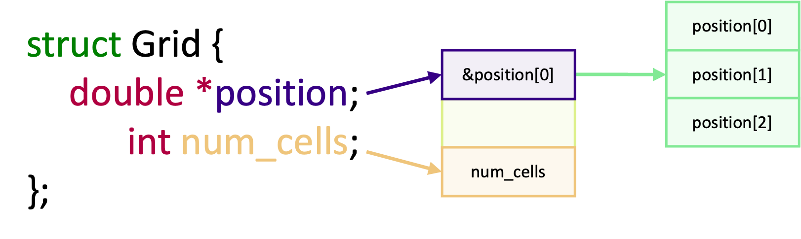
A different way to calculate displacements
There are other ways to calculate the displacement, other than using what MPI provides for us. Another common way is to use the
offsetof()macro part of<stddef.h>.offsetof()accepts two arguments, the first being the struct type and the second being the member to calculate the offset for.#include <stddef.h> MPI_Aint displacements[2]; displacements[0] = (MPI_Aint) offsetof(struct MyStruct, id); // The cast to MPI_Aint is for extra safety displacements[1] = (MPI_Aint) offsetof(struct MyStruct, value);This method and the other shown in the previous examples both returns the same displacement values. It’s mostly a personal choice which you choose to use. Some people prefer the “safety” of using
MPI_Get_address()whilst others prefer to write more concise code withoffsetof(). Of course, if you’re a Fortran programmer then you can’t use the macro!
Complex non-contiguous and heterogeneous data
The previous two sections covered how to communicate complex but structured data between ranks using derived datatypes.
However, there are always some edge cases which don’t fit into a derived types. For example, just in the last exercise
we’ve seen that pointers and derived types don’t mix well. Furthermore, we can sometimes also reach performance
bottlenecks when working with heterogeneous data which doesn’t fit, or doesn’t make sense to be, in a derived type, as
each data type needs to be communicated in separate communication calls. This can be especially bad if blocking
communication is used! For edge cases situations like this, we can use the MPI_Pack() and MPI_Unpack() functions to
do things ourselves.
Both MPI_Pack() and MPI_Unpack() are methods for manually arranging, packing and unpacking data into a contiguous
buffer, for cases where regular communication methods and derived types don’t work well or efficiently. They can also be
used to create self-documenting message, where the packed data contains additional elements which describe the size,
structure and contents of the data. But we have to be careful, as using packed buffers comes with additional overhead,
in the form of increased memory usage and potentially more communication overhead as packing and unpacking data is not
free.
When we use MPI_Pack(), we take non-contiguous data (sometimes of different datatypes) and “pack” it into a
contiguous memory buffer. The diagram below shows how two (non-contiguous) chunks of data may be packed into a contiguous
array using MPI_Pack().

The coloured boxes in both memory representations (memory and pakced) are the same chunks of data. The green boxes
containing only a single number are used to document the number of elements in the block of elements they are adjacent
to, in the contiguous buffer. This is optional to do, but is generally good practise to include to create a
self-documenting message. From the diagram we can see that we have “packed” non-contiguous blocks of memory into a
single contiguous block. We can do this using MPI_Pack(). To reverse this action, and “unpack” the buffer, we use
MPI_Unpack(). As you might expect, MPI_Unpack() takes a buffer, created by MPI_Pack() and unpacks the data back
into various memory address.
To pack data into a contiguous buffer, we have to pack each block of data, one by one, into the contiguous buffer using
the MPI_Pack() function,
int MPI_Pack(
   const void *inbuf,
   int incount,
   MPI_Datatype datatype,
   void *outbuf,
   int outsize,
   int *position,
   MPI_Comm comm
);
*inbuf: |
The data to pack into the buffer |
incount: |
The number of elements to pack |
datatype: |
The data type of the data to pack |
*outbuf: |
The out buffer of contiguous data |
outsize: |
The size of the out buffer, in bytes |
*position: |
A counter for how far into the contiguous buffer to write (records the position, in bytes) |
comm: |
The communicator |
In the above, inbuf is the data we want to pack into a contiguous buffer and incount and datatype define the
number of elements in and the datatype of inbuf. The parameter outbuf is the contiguous buffer the data is packed
into, with outsize being the total size of the buffer in bytes. The position argument is used to keep track of the
current position, in bytes, where data is being packed into outbuf.
Uniquely, MPI_Pack(), and MPI_Unpack() as well, measure the size of the contiguous buffer, outbuf, in bytes rather than
in number of elements. Given that MPI_Pack() is all about manually arranging data, we have to also manage the
allocation of memory for outbuf. But how do we allocate memory for it, and how much should we allocate? Allocation is
done by using malloc(). Since MPI_Pack() works with outbuf in terms of bytes, the convention is to declare
outbuf as a char *. The amount of memory to allocate is simply the amount of space, in bytes, required to store all
of the data we want to pack into it. Just like how we would normally use malloc() to create an array. If we had
an integer array and a floating point array which we wanted to pack into the buffer, then the size required is easy to
calculate,
// The total buffer size is the sum of the bytes required for the int and float array
int size_int_array = num_int_elements * sizeof(int);
int size_float_array = num_float_elements * sizeof(float);
int buffer_size = size_int_array + size_float_array;
// The buffer is a char *, but could also be cast as void * if you prefer
char *buffer = malloc(buffer_size * sizeof(char));  // a char is 1 byte, so sizeof(char) is optional
If we are also working with derived types, such as vectors or structs, then we need to find the size of those types. By
far the easiest way to handle these is to use MPI_Pack_size(), which supports derived datatypes through the
MPI_Datatype,
nt MPI_Pack_size(
   int incount,
   MPI_Datatype datatype,
   MPI_Comm comm,
   int *size
);
incount: |
The number of data elements |
datatype: |
The data type of the data |
comm: |
The communicator |
*size: |
The calculated upper size limit for the buffer, in bytes |
MPI_Pack_size() is a helper function to calculate the upper bound of memory required. It is, in general, preferable
to calculate the buffer size using this function, as it takes into account any implementation specific MPI detail and
thus is more portable between implementations and systems. If we wanted to calculate the memory required for three
elements of some derived struct type and a double array, we would do the following,
int struct_array_size, float_array_size;
MPI_Pack_size(3, STRUCT_DERIVED_TYPE, MPI_COMM_WORLD, &struct_array_size);
MPI_Pack_size(50, MPI_DOUBLE. MPI_COMM_WORLD, &float_array_size);
int buffer_size = struct_array_size + float_array_size;
When a rank has received a contiguous buffer, it has to be unpacked into its constituent parts, one by one, using
MPI_Unpack(),
int MPI_Unpack(
   void *inbuf,
   int insize,
   int *position,
   void *outbuf,
   int outcount,
   MPI_Datatype datatype,
   MPI_Comm comm,
);
*inbuf: |
The contiguous buffer to unpack |
insize: |
The total size of the buffer, in bytes |
*position: |
The position, in bytes, from where to start unpacking from |
*outbuf: |
An array, or variable, to unpack data into – this is the output |
outcount: |
The number of elements of data to unpack |
datatype: |
The data type of elements to unpack |
comm: |
The communicator |
The arguments for this function are essentially the reverse of MPI_Pack(). Instead of being the buffer to pack into,
inbuf is now the packed buffer and position is the position, in bytes, in the buffer where to unpacking from.
outbuf is then the variable we want to unpack into, and outcount is the number of elements of datatype to unpack.
In the example below, MPI_Pack(), MPI_Pack_size() and MPI_Unpack() are used to communicate a (non-contiguous)
3 x 3 matrix.
// Allocate and initialise a (non-contiguous) 2D matrix that we will pack into
// a buffer
int num_rows = 3, num_cols = 3;
int **matrix = malloc(num_rows * sizeof(int *));
for (int i = 0; i < num_rows; ++i) {
   matrix[i] = malloc(num_cols * sizeof(int));
   for (int j = 0; i < num_cols; ++j) {
      matrix[i][j] = num_cols * i + j;
   }
}

// Determine the upper limit for the amount of memory the buffer requires. Since
// this is a simple situation, we could probably have done this manually using
// `num_rows * num_cols * sizeof(int)`. The size `pack_buffer_size` is returned in
// bytes
int pack_buffer_size;
MPI_Pack_size(num_rows * num_cols, MPI_INT, MPI_COMM_WORLD, &pack_buffer_size);

if (my_rank == 0) {
    // Create the pack buffer and pack each row of data into it buffer
    // one by one
    int position = 0;
    char *packed_data = malloc(pack_buffer_size);
    for (int i = 0; i < num_rows; ++i) {
        MPI_Pack(matrix[i], num_cols, MPI_INT, packed_data, pack_buffer_size, &position, MPI_COMM_WORLD);
    }

    // Send the packed data to rank 1
    MPI_Send(packed_data, pack_buffer_size, MPI_PACKED, 1, 0, MPI_COMM_WORLD);
} else {
    // Create a receive buffer and get the packed buffer from rank 0
    char *received_data = malloc(pack_buffer_size);
    MPI_Recv(received_data, pack_buffer_size + 1, MPI_PACKED, 0, 0, MPI_COMM_WORLD, MPI_STATUS_IGNORE);

    // Allocate a matrix to put the receive buffer into -- this is for demonstration purposes
    int **my_matrix = malloc(num_rows * sizeof(int *));
    for (int i = 0; i < num_cols; ++i) {
        my_matrix[i] = malloc(num_cols * sizeof(int));
    }

    // Unpack the received data row by row into my_matrix
    int position = 0;
    for (int i = 0; i < num_rows; ++i) {
        MPI_Unpack(received_data, pack_buffer_size, &position, my_matrix[i], num_cols, MPI_INT, MPI_COMM_WORLD);
    }
}
Blocking or non-blocking?
The processes of packing data into a contiguous buffer does not happen asynchronously. The same goes for unpacking data. But this doesn’t restrict the packed data from being only sent synchronously. The packed data can be communicated using any communication function, just like the previous derived types. It works just as well to communicate the buffer using non-blocking methods, as it does using blocking methods.
What if the other rank doesn’t know the size of the buffer?
In some cases, the receiving rank may not know the size of the buffer used in
MPI_Pack(). This could happen if a message is sent and received in different functions, if some ranks have different branches through the program or if communication happens in a dynamic or non-sequential way.In these situations, we can use
MPI_Probe()andMPI_Get_countto find the a message being sent and to get the number of elements in the message.// First probe for a message, to get the status of it MPI_Status status; MPI_Probe(0, 0, MPI_COMM_WORLD, &status); // Using MPI_Get_count we can get the number of elements of a particular data type int message_size; MPI_Get_count(&status, MPI_PACKED, &buffer_size); // MPI_PACKED represents an element of a "byte stream." So, buffer_size is the size of the buffer to allocate char *buffer = malloc(buffer_size);
Sending heterogeneous data in a single communication
Suppose we have two arrays below, where one contains integer data and the other floating point data. Normally we would use multiple communication calls to send each type of data individually, for a known number of elements. For this exercise, communicate both arrays using a packed memory buffer.
int int_data_count = 5;
int float_data_count = 10;

int   *int_data = malloc(int_data_count * sizeof(int));
float *float_data = malloc(float_data_count * sizeof(float));

// Initialize the arrays with some values
for (int i = 0; i < int_data_count; ++i) {
  int_data[i] = i + 1;
}
for (int i = 0; i < float_data_count; ++i) {
  float_data[i] = 3.14159 * (i + 1);
}
Since the arrays are dynamically allocated, in rank 0, you should also pack the number of elements in each array. Rank 1 may also not know the size of the buffer. How would you deal with that?
You can use this skeleton code to begin with.
Solution
The additional restrictions for rank 1 not knowing the size of the arrays or packed buffer add some complexity to receiving the packed buffer from rank 0.
#include <mpi.h>
#include <stdio.h>
#include <stdlib.h>

int main(int argc, char **argv)
{
    int my_rank;
    int num_ranks;
    MPI_Init(&argc, &argv);
    MPI_Comm_rank(MPI_COMM_WORLD, &my_rank);
    MPI_Comm_size(MPI_COMM_WORLD, &num_ranks);

    if (num_ranks != 2) {
        if (my_rank == 0) {
            printf("This example only works with 2 ranks\n");
        }
        MPI_Abort(MPI_COMM_WORLD, 1);
    }

    if (my_rank == 0) {
        int int_data_count = 5, float_data_count = 10;
        int *int_data = malloc(int_data_count * sizeof(int));
        float *float_data = malloc(float_data_count * sizeof(float));
        for (int i = 0; i < int_data_count; ++i) {
            int_data[i] = i + 1;
        }
        for (int i = 0; i < float_data_count; ++i) {
            float_data[i] = 3.14159 * (i + 1);
        }

        // use MPI_Pack_size to determine how big the packed buffer needs to be
        int buffer_size_count, buffer_size_int, buffer_size_float;
        MPI_Pack_size(2, MPI_INT, MPI_COMM_WORLD, &buffer_size_count); // 2 * INT because we will have 2 counts
        MPI_Pack_size(int_data_count, MPI_INT, MPI_COMM_WORLD, &buffer_size_int);
        MPI_Pack_size(float_data_count, MPI_FLOAT, MPI_COMM_WORLD, &buffer_size_float);
        int total_buffer_size = buffer_size_int + buffer_size_float + buffer_size_count;

        int position = 0;
        char *buffer = malloc(total_buffer_size);

        // Pack the data size, followed by the actually data
        MPI_Pack(&int_data_count, 1, MPI_INT, buffer, total_buffer_size, &position, MPI_COMM_WORLD);
        MPI_Pack(int_data, int_data_count, MPI_INT, buffer, total_buffer_size, &position, MPI_COMM_WORLD);
        MPI_Pack(&float_data_count, 1, MPI_INT, buffer, total_buffer_size, &position, MPI_COMM_WORLD);
        MPI_Pack(float_data, float_data_count, MPI_FLOAT, buffer, total_buffer_size, &position, MPI_COMM_WORLD);

        // buffer is sent in one communication using MPI_PACKED
        MPI_Send(buffer, total_buffer_size, MPI_PACKED, 1, 0, MPI_COMM_WORLD);

        free(buffer);
        free(int_data);
        free(float_data);
    } else {
        int buffer_size;
        MPI_Status status;
        MPI_Probe(0, 0, MPI_COMM_WORLD, &status);
        MPI_Get_count(&status, MPI_PACKED, &buffer_size);

        char *buffer = malloc(buffer_size);
        MPI_Recv(buffer, buffer_size, MPI_PACKED, 0, 0, MPI_COMM_WORLD, &status);

        int position = 0;
        int int_data_count, float_data_count;

        // Unpack an integer why defines the size of the integer array,
        // then allocate space for an unpack the actual array
        MPI_Unpack(buffer, buffer_size, &position, &int_data_count, 1, MPI_INT, MPI_COMM_WORLD);
        int *int_data = malloc(int_data_count * sizeof(int));
        MPI_Unpack(buffer, buffer_size, &position, int_data, int_data_count, MPI_INT, MPI_COMM_WORLD);

        MPI_Unpack(buffer, buffer_size, &position, &float_data_count, 1, MPI_INT, MPI_COMM_WORLD);
        float *float_data = malloc(float_data_count * sizeof(float));
        MPI_Unpack(buffer, buffer_size, &position, float_data, float_data_count, MPI_FLOAT, MPI_COMM_WORLD);

        printf("int data: [");
        for (int i = 0; i < int_data_count; ++i) {
            printf(" %d", int_data[i]);
        }
        printf(" ]\n");

        printf("float data: [");
        for (int i = 0; i < float_data_count; ++i) {
            printf(" %f", float_data[i]);
        }
        printf(" ]\n");

        free(int_data);
        free(float_data);
        free(buffer);
    }

    return MPI_Finalize();
}
Key Points
Structures can be communicated easier by using
MPI_Type_create_structto create a derived type describing the structureThe functions
MPI_Pack()andMPI_Unpack()can be used to manually create a contiguous memory block of data, to communicate complex and/or heterogeneous data structures
Survey
Overview
Teaching: min
Exercises: minQuestions
Objectives
Key Points